library("tidyverse")

library("lubridate")

library("ggpubr")

library("summarytools")

# The libraries "HydroTSM", "descr", "DT", "SemTools" are also used R Real Estate Project
Introduction
This project aims to examine national real estate data using R with several variables, including potential subgroups based on location or date and relationships between several variables (visually and through an appropriate hypothesis test).
Resources
I visited the website https://www.realtor.com/research/data/ and found the following CSV file to examine.
- RDC_Inventory_Core_Metrics_State_History.csv
Step 1 - Read in, Clean, and Prepare Data
Read in Libraries
Read in Dataset
I used summary() and head() to check for NAs and ensure no extra rows were up top.
State <- read.csv("data/RDC_Inventory_Core_Metrics_State_History.csv")

# summary(State)

# head(State)

# I commented out printing the top rows and summary stats for cleanliness in output
# Summary of State for Web
print(dfSummary(State,
varnumbers = FALSE,
valid.col = FALSE,
graph.magnif = 0.76),
max.tbl.height = 400,
method = 'render')Data Frame Summary
State
Dimensions: 3775 x 40Duplicates: 0
| Variable | Stats / Values | Freqs (% of Valid) | Graph | Missing | |||||||||||||||||||||||||||||||||||||||||||||||||||||||
|---|---|---|---|---|---|---|---|---|---|---|---|---|---|---|---|---|---|---|---|---|---|---|---|---|---|---|---|---|---|---|---|---|---|---|---|---|---|---|---|---|---|---|---|---|---|---|---|---|---|---|---|---|---|---|---|---|---|---|---|
| month_date_yyyymm [integer] |
|
74 distinct values |  |
0 (0.0%) | |||||||||||||||||||||||||||||||||||||||||||||||||||||||
| state [character] |
|
|
 |
0 (0.0%) | |||||||||||||||||||||||||||||||||||||||||||||||||||||||
| state_id [character] |
|
|
|
0 (0.0%) | |||||||||||||||||||||||||||||||||||||||||||||||||||||||
| median_listing_price [integer] |
|
1851 distinct values |  |
0 (0.0%) | |||||||||||||||||||||||||||||||||||||||||||||||||||||||
| median_listing_price_mm [numeric] |
|
922 distinct values |  |
613 (16.2%) | |||||||||||||||||||||||||||||||||||||||||||||||||||||||
| median_listing_price_yy [numeric] |
|
1688 distinct values |  |
613 (16.2%) | |||||||||||||||||||||||||||||||||||||||||||||||||||||||
| active_listing_count [integer] |
|
3584 distinct values |  |
0 (0.0%) | |||||||||||||||||||||||||||||||||||||||||||||||||||||||
| active_listing_count_mm [numeric] |
|
1972 distinct values |  |
613 (16.2%) | |||||||||||||||||||||||||||||||||||||||||||||||||||||||
| active_listing_count_yy [numeric] |
|
2554 distinct values |  |
613 (16.2%) | |||||||||||||||||||||||||||||||||||||||||||||||||||||||
| median_days_on_market [integer] |
|
154 distinct values |  |
0 (0.0%) | |||||||||||||||||||||||||||||||||||||||||||||||||||||||
| median_days_on_market_mm [numeric] |
|
1737 distinct values |  |
613 (16.2%) | |||||||||||||||||||||||||||||||||||||||||||||||||||||||
| median_days_on_market_yy [numeric] |
|
1866 distinct values |  |
613 (16.2%) | |||||||||||||||||||||||||||||||||||||||||||||||||||||||
| new_listing_count [integer] |
|
2480 distinct values |  |
0 (0.0%) | |||||||||||||||||||||||||||||||||||||||||||||||||||||||
| new_listing_count_mm [numeric] |
|
2451 distinct values |  |
613 (16.2%) | |||||||||||||||||||||||||||||||||||||||||||||||||||||||
| new_listing_count_yy [numeric] |
|
2176 distinct values |  |
613 (16.2%) | |||||||||||||||||||||||||||||||||||||||||||||||||||||||
| price_increased_count [integer] |
|
731 distinct values |  |
0 (0.0%) | |||||||||||||||||||||||||||||||||||||||||||||||||||||||
| price_increased_count_mm [numeric] |
|
1962 distinct values |  |
613 (16.2%) | |||||||||||||||||||||||||||||||||||||||||||||||||||||||
| price_increased_count_yy [numeric] |
|
2144 distinct values |  |
613 (16.2%) | |||||||||||||||||||||||||||||||||||||||||||||||||||||||
| price_reduced_count [integer] |
|
2020 distinct values |  |
0 (0.0%) | |||||||||||||||||||||||||||||||||||||||||||||||||||||||
| price_reduced_count_mm [numeric] |
|
2537 distinct values |  |
613 (16.2%) | |||||||||||||||||||||||||||||||||||||||||||||||||||||||
| price_reduced_count_yy [numeric] |
|
2702 distinct values |  |
613 (16.2%) | |||||||||||||||||||||||||||||||||||||||||||||||||||||||
| pending_listing_count [integer] |
|
3306 distinct values |  |
21 (0.6%) | |||||||||||||||||||||||||||||||||||||||||||||||||||||||
| pending_listing_count_mm [numeric] |
|
2219 distinct values |  |
633 (16.8%) | |||||||||||||||||||||||||||||||||||||||||||||||||||||||
| pending_listing_count_yy [numeric] |
|
2713 distinct values |  |
643 (17.0%) | |||||||||||||||||||||||||||||||||||||||||||||||||||||||
| median_listing_price_per_square_foot [integer] |
|
393 distinct values |  |
0 (0.0%) | |||||||||||||||||||||||||||||||||||||||||||||||||||||||
| median_listing_price_per_square_foot_mm [numeric] |
|
684 distinct values |  |
613 (16.2%) | |||||||||||||||||||||||||||||||||||||||||||||||||||||||
| median_listing_price_per_square_foot_yy [numeric] |
|
1708 distinct values |  |
613 (16.2%) | |||||||||||||||||||||||||||||||||||||||||||||||||||||||
| median_square_feet [integer] |
|
972 distinct values |  |
0 (0.0%) | |||||||||||||||||||||||||||||||||||||||||||||||||||||||
| median_square_feet_mm [numeric] |
|
602 distinct values |  |
613 (16.2%) | |||||||||||||||||||||||||||||||||||||||||||||||||||||||
| median_square_feet_yy [numeric] |
|
1296 distinct values |  |
613 (16.2%) | |||||||||||||||||||||||||||||||||||||||||||||||||||||||
| average_listing_price [integer] |
|
3764 distinct values |  |
0 (0.0%) | |||||||||||||||||||||||||||||||||||||||||||||||||||||||
| average_listing_price_mm [numeric] |
|
905 distinct values |  |
613 (16.2%) | |||||||||||||||||||||||||||||||||||||||||||||||||||||||
| average_listing_price_yy [numeric] |
|
1819 distinct values |  |
613 (16.2%) | |||||||||||||||||||||||||||||||||||||||||||||||||||||||
| total_listing_count [integer] |
|
3634 distinct values |  |
0 (0.0%) | |||||||||||||||||||||||||||||||||||||||||||||||||||||||
| total_listing_count_mm [numeric] |
|
1833 distinct values |  |
613 (16.2%) | |||||||||||||||||||||||||||||||||||||||||||||||||||||||
| total_listing_count_yy [numeric] |
|
2345 distinct values |  |
613 (16.2%) | |||||||||||||||||||||||||||||||||||||||||||||||||||||||
| pending_ratio [numeric] |
|
3191 distinct values |  |
21 (0.6%) | |||||||||||||||||||||||||||||||||||||||||||||||||||||||
| pending_ratio_mm [numeric] |
|
1774 distinct values |  |
633 (16.8%) | |||||||||||||||||||||||||||||||||||||||||||||||||||||||
| pending_ratio_yy [numeric] |
|
2443 distinct values |  |
640 (17.0%) | |||||||||||||||||||||||||||||||||||||||||||||||||||||||
| quality_flag [integer] |
|
|
 |
612 (16.2%) |
Generated by summarytools 1.0.1 (R version 4.4.1)
2024-11-01
# Print top 5 rows in web-friendly format
DT::datatable(head(State))
Clean Data
State.cleaned <- State %>%

     mutate(month_date_yyyymm = as.character(month_date_yyyymm)) %>%

     rename(date = month_date_yyyymm) %>%

     mutate(date = ym(date)) %>%

     mutate(state = as.factor(state)) %>%

     mutate(state_id = as.factor(state_id)) %>%

     mutate(median_listing_price = as.numeric(median_listing_price)) %>%

     mutate(monthly_new_listing_count = new_listing_count * 4) %>%

     # needed to adjust above because it was in weekly units (everything else in monthly)

     mutate(quality_flag = recode_factor(.x = quality_flag,

                                         `1` = "yes",

                                         `0` = "no"))

# tail(State.cleaned)

# I used tail to make sure there were no extra rows on bottom. This is commented
# out to not clutter the output in the PDF.

###############

# Create the region classifications

NE.name <- c("Connecticut", "Maine", "Massachusetts", "New Hampshire",

             "Rhode Island", "Vermont", "New Jersey", "New York",

             "Pennsylvania")

NE.abrv <- c("CT", "ME", "MA", "NH", "RI", "VT", "NJ", "NY", "PA")

NE.ref <- c(NE.name,NE.abrv)

MW.name <- c("Indiana", "Illinois", "Michigan", "Ohio", "Wisconsin",

             "Iowa", "Kansas", "Minnesota", "Missouri", "Nebraska",

             "North Dakota", "South Dakota")

MW.abrv <- c("IN", "IL", "MI", "OH", "WI", "IA", "KS", "MN", "MO", "NE",

             "ND", "SD")

MW.ref <- c(MW.name,MW.abrv)

SE.name <- c("Arkansas", "Louisiana", "Alabama", "Kentucky", "Mississippi",

             "Tennessee", "District of Columbia", "Florida", "Georgia",

             "Delaware", "Maryland", "North Carolina", "South Carolina",

             "Virginia", "West Virginia")

SE.abrv <- c("AR","LA", "AL", "KY", "MS", "TN", "DC", "FL", "GA", "DE", "MD",

             "NC", "SC", "VA", "WV")

SE.ref <- c(SE.name,SE.abrv)

SW.name <- c("Arizona", "New Mexico", "Texas", "Oklahoma")

SW.abrv <- c("AZ", "NM", "TX", "OK")

SW.ref <- c(SW.name,SW.abrv)

W.name <- c("Washington", "Oregon", "California", "Montana", "Idaho","Nevada",

            "Wyoming", "Utah", "Colorado", "Hawaii", "Alaska")

W.abrv <- c("WA", "OR", "CA", "MT", "ID", "NV", "WY", "UT", "CO", "HI", "AK")

W.ref <- c(W.name,W.abrv)

region.list <- list(Northeast = NE.ref,

                    Midwest = MW.ref,

                    Southwest = SW.ref,

                    Southeast = SE.ref,

                    West = W.ref)

# Map Source - https://education.nationalgeographic.org/resource/united-states-regions/

###############

small.list <- State.cleaned %>%

     select(active_listing_count, median_listing_price,

            median_days_on_market, monthly_new_listing_count,

            median_square_feet, pending_listing_count,

            date, state, state_id) %>%

     mutate(month = as.factor(format(date, "%m")),

            year = as.factor(format(date, "%Y"))) %>%

     subset(state != "marshall islands") %>%

     # removing Marshall Islands because it has NAs and throws off rest of numbers
     # plus, the Marshall Islands are not part of the geographic region I want to analyze

     mutate(state_id = as.factor(toupper(state_id))) %>%

     mutate(across(where(is.factor), str_trim)) %>%

     mutate(seasons = hydroTSM::time2season(date, out.fmt = "seasons")) %>%

     mutate(region = sapply(state_id,

                     function(x) names(region.list)[grep(x, region.list)])) %>%

     mutate_if(is.character, as.factor)


# summary(small.list)

# Same as above. Just checked re-coding to make sure it worked properly.
# Commented out for web
# Summary of State for Web
print(dfSummary(small.list,
varnumbers = FALSE,
valid.col = FALSE,
graph.magnif = 0.76),
max.tbl.height = 400,
method = 'render')Data Frame Summary
small.list
Dimensions: 3774 x 13Duplicates: 0
| Variable | Stats / Values | Freqs (% of Valid) | Graph | Missing | |||||||||||||||||||||||||||||||||||||||||||||||||||||||
|---|---|---|---|---|---|---|---|---|---|---|---|---|---|---|---|---|---|---|---|---|---|---|---|---|---|---|---|---|---|---|---|---|---|---|---|---|---|---|---|---|---|---|---|---|---|---|---|---|---|---|---|---|---|---|---|---|---|---|---|
| active_listing_count [integer] |
|
3583 distinct values |  |
0 (0.0%) | |||||||||||||||||||||||||||||||||||||||||||||||||||||||
| median_listing_price [numeric] |
|
1850 distinct values |  |
0 (0.0%) | |||||||||||||||||||||||||||||||||||||||||||||||||||||||
| median_days_on_market [integer] |
|
153 distinct values |  |
0 (0.0%) | |||||||||||||||||||||||||||||||||||||||||||||||||||||||
| monthly_new_listing_count [numeric] |
|
2479 distinct values |  |
0 (0.0%) | |||||||||||||||||||||||||||||||||||||||||||||||||||||||
| median_square_feet [integer] |
|
971 distinct values |  |
0 (0.0%) | |||||||||||||||||||||||||||||||||||||||||||||||||||||||
| pending_listing_count [integer] |
|
3306 distinct values |  |
20 (0.5%) | |||||||||||||||||||||||||||||||||||||||||||||||||||||||
| date [Date] |
|
74 distinct values |  |
0 (0.0%) | |||||||||||||||||||||||||||||||||||||||||||||||||||||||
| state [factor] |
|
|
 |
0 (0.0%) | |||||||||||||||||||||||||||||||||||||||||||||||||||||||
| state_id [factor] |
|
|
|
0 (0.0%) | |||||||||||||||||||||||||||||||||||||||||||||||||||||||
| month [factor] |
|
|
 |
0 (0.0%) | |||||||||||||||||||||||||||||||||||||||||||||||||||||||
| year [factor] |
|
|
 |
0 (0.0%) | |||||||||||||||||||||||||||||||||||||||||||||||||||||||
| seasons [factor] |
|
|
 |
0 (0.0%) | |||||||||||||||||||||||||||||||||||||||||||||||||||||||
| region [factor] |
|
|
 |
0 (0.0%) |
Generated by summarytools 1.0.1 (R version 4.4.1)
2024-11-01
Step 2 - Examine Variables
Here, I examine several variables from the data set, including measures of central tendency and spread for continuous variables and frequency and relative frequency for categorical variables.
- Months (categorical)
- Years (categorical)
- Regions (categorical)
- Seasons (categorical)
- Active Listing Count (continuous)
- Median Listing Price (continuous)
- Median Days on Market (continuous)
- New Listing Count Monthly (continuous)
- Median Square Feet (continuous)
- Pending Listing Count (continuous)(this one has NA for AK)
A. Months (categorical)
descr::freq(small.list$month, plot = F)small.list$month
Frequency Percent
01 306 8.108
02 306 8.108
03 306 8.108
04 306 8.108
05 306 8.108
06 306 8.108
07 357 9.459
08 357 9.459
09 306 8.108
10 306 8.108
11 306 8.108
12 306 8.108
Total 3774 100.000Comments -
All the months have the same observations (306) other than July and August (357).
B. Years (categorical)
descr::freq(small.list$year, plot = F)small.list$year
Frequency Percent
2016 306 8.108
2017 612 16.216
2018 612 16.216
2019 612 16.216
2020 612 16.216
2021 612 16.216
2022 408 10.811
Total 3774 100.000Comments -
All the years have the same observations (612) other than 2016 (306) and 2022 (408).
C. Regions (categorical)
descr::freq(small.list$region, plot = F)small.list$region
Frequency Percent
Midwest 888 23.529
Northeast 666 17.647
Southeast 1110 29.412
Southwest 296 7.843
West 814 21.569
Total 3774 100.000Comments -
Looking at the table, you see that the Southeast has the most observations. This does make sense, given that the Southeast has the most states in that category (15). The order in terms of number of states in the regions is Southeast (15), Midwest (12), West (11), Northeast (9), and finally Southwest (4). The table of frequencies follows this pattern as well from greatest to least. However, this should not matter as much when we do calculations by median later.
D. Seasons (categorical)
descr::freq(small.list$seasons, plot = F)small.list$seasons
Frequency Percent
autumn 918 24.32
spring 918 24.32
summer 1020 27.03
winter 918 24.32
Total 3774 100.00Comments -
Summer has the most observations here, which makes sense given that July and August had more observations (noted earlier). As I mentioned above, we can account for this when we do calculations later.
1. Active Listing Count (continuous)
small.list %>%

     summarise(mean.active = mean(active_listing_count),

               sd.active = sd(active_listing_count),

               med.active = median(active_listing_count),

               iqr.active = IQR(active_listing_count),

               mode.active = names(sort(table(active_listing_count),

decreasing = TRUE))[1]) semTools::skew(small.list$active_listing_count) skew (g1) se z p
2.69424610 0.03987261 67.57134854 0.00000000 2. Median Listing Price (continuous)
small.list %>%

     summarise(mean.price = mean(median_listing_price),

               sd.price = sd(median_listing_price),

               med.price = median(median_listing_price),

               iqr.price = IQR(median_listing_price),

               mode.price = names(sort(table(median_listing_price),

decreasing = TRUE))[1]) semTools::skew(small.list$median_listing_price) skew (g1) se z p
1.21345068 0.03987261 30.43318832 0.00000000 3. Median Days on Market (continuous)
small.list %>%

     summarise(mean.days.mkt = mean(median_days_on_market),

               sd.days.mkt = sd(median_days_on_market),

               med.days.mkt = median(median_days_on_market),

               iqr.days.mkt = IQR(median_days_on_market),

               mode.days.mkt = names(sort(table(median_days_on_market),

decreasing = TRUE))[1]) semTools::skew(small.list$median_days_on_market) skew (g1) se z p
1.06096887 0.03987261 26.60896395 0.00000000 4. New Listing Count Monthly (continuous)
small.list %>%

     summarise(mean.new.list.num = mean(monthly_new_listing_count),

               sd.new.list.num = sd(monthly_new_listing_count),

               med.new.list.num = median(monthly_new_listing_count),

               iqr.new.list.num = IQR(monthly_new_listing_count),

               mode.new.list.num = names(sort(table(monthly_new_listing_count),

decreasing = TRUE))[1]) semTools::skew(small.list$monthly_new_listing_count) skew (g1) se z p
2.19673355 0.03987261 55.09379710 0.00000000 5. Median Square Feet (continuous)
small.list %>%

     summarise(mean.sq.ft = mean(median_square_feet),

               sd.sq.ft = sd(median_square_feet),

               med.sq.ft = median(median_square_feet),

               iqr.sq.ft = IQR(median_square_feet),

               mode.sq.ft = names(sort(table(median_square_feet),

decreasing = TRUE))[1]) semTools::skew(small.list$median_square_feet) skew (g1) se z p
-1.828905e-01 3.987261e-02 -4.586871e+00 4.499375e-06 6. Pending Listing Count (continuous)(this one has NA for AK)
small.list %>%

     drop_na() %>%

     summarise(mean.pend.num = mean(pending_listing_count),

               sd.pend.num = sd(pending_listing_count),

               med.pend.num = median(pending_listing_count),

               iqr.pend.num = IQR(pending_listing_count),

               mode.pend.num = names(sort(table(pending_listing_count),

decreasing = TRUE))[1]) semTools::skew(small.list$pending_listing_count) skew (g1) se z p
2.57162812 0.03997868 64.32498236 0.00000000 Overall Continuous Variable Comments
Comments -
Most of these variables (except Median sq ft) had a problem with skewness. All of the variables that were skewed were positively skewed (Mode < Median < Mean). Since most of the data is very positively skewed, the median or mode would be best to look at rather than the mean for everything except the median sq ft data.
Otherwise, the summary statistics I gathered in this section were that in the US, the median number of active listings is 11895, with an IQR of 19198.5 listings. The mean is 20157.7, with an even higher standard deviation of 23970.85 listings. The mode was 2826 listings.
The median number of monthly median listing price is $290,358 with an IQR of $144,971.50. The mean is $325,052.90, with a standard deviation of $129,990.10. The mode was $299,900.
The median number of days on the market is 64 days, with an IQR of 32 days. The mean is 66.37 days with a standard deviation of 25 days. The mode was 64 days.
The median number of monthly new listings on the market is 22000 with an IQR of 36224. The mean is 35187.44, with a standard deviation of 39378.73 listings. The mode was 4816.
Since the median square feet data is more normally distributed, we can look at the mean first. The mean square feet is 1925.015 with a standard deviation of 241.4007 sq ft. The mode is 1800 sq ft. The median is 1936, with an IQR of 256 sq ft.
The pending listing count is the only variable with NA values (listed for Alaska). Otherwise, this data is also positively skewed, and the median number of pending listings on the market is 5330.5 with an IQR of 10186.25. The mean is 9623.955, with a standard deviation of 12488.11 listings. The mode was 68 listings.
Step 3 - Group Data for Further Exploration
This section will be sorted by state in a few ways.
Descending Price by State
small.list %>%

     group_by(state, region) %>%

     summarise(med.price = median(median_listing_price),

               mean.sq.ft = mean(median_square_feet),

               med.active = median(active_listing_count),

               med.pending = median(pending_listing_count, na.rm = T),

               med.days.mkt = median(median_days_on_market),

               med.new.listing = median(monthly_new_listing_count)) %>%

     arrange(desc(med.price))
Descending Mean Sq Ft by State
small.list %>%

     group_by(state, region) %>%

     summarise(med.price = median(median_listing_price),

               mean.sq.ft = mean(median_square_feet),

               med.active = median(active_listing_count),

               med.pending = median(pending_listing_count, na.rm = T),

               med.days.mkt = median(median_days_on_market),

               med.new.listing = median(monthly_new_listing_count)) %>%

     arrange(desc(mean.sq.ft))
Descending Median Days on Market by State
small.list %>%

     group_by(state, region) %>%

     summarise(med.price = median(median_listing_price),

               mean.sq.ft = mean(median_square_feet),

               med.active = median(active_listing_count),

               med.pending = median(pending_listing_count, na.rm = T),

               med.days.mkt = median(median_days_on_market),

               med.new.listing = median(monthly_new_listing_count)) %>%

     arrange(desc(med.days.mkt))
Ascending Median Days on Market by State
small.list %>%

     group_by(state, region) %>%

     summarise(med.price = median(median_listing_price),

               mean.sq.ft = mean(median_square_feet),

               med.active = median(active_listing_count),

               med.pending = median(pending_listing_count, na.rm = T),

               med.days.mkt = median(median_days_on_market),

               med.new.listing = median(monthly_new_listing_count)) %>%

arrange(med.days.mkt)Grouped by Month
small.list %>%

     group_by(month) %>%

     summarise(med.price = median(median_listing_price),

               mean.sq.ft = mean(median_square_feet),

               med.active = median(active_listing_count),

               med.pending = median(pending_listing_count, na.rm = T),

               med.days.mkt = median(median_days_on_market),

               med.new.listing = median(monthly_new_listing_count))
Descending Price by Month
small.list %>%

     group_by(month) %>%

     summarise(med.price = median(median_listing_price),

               mean.sq.ft = mean(median_square_feet),

               med.active = median(active_listing_count),

               med.pending = median(pending_listing_count, na.rm = T),

               med.days.mkt = median(median_days_on_market),

               med.new.listing = median(monthly_new_listing_count)) %>%

     arrange(desc(med.price))
Comments on by Month Grouping
It seems to be seasonal (more comments are in the seasonality section). June has the highest prices, with December having the lowest. February through April also had the lowest active listings but the same amount (roughly) of pending and new listings as other months. December through February also had the longest median on the market values as well.
Descending Price by Year
small.list %>%

     group_by(year) %>%

     summarise(med.price = median(median_listing_price),

               mean.sq.ft = mean(median_square_feet),

               med.active = median(active_listing_count),

               med.pending = median(pending_listing_count, na.rm = T),

               med.days.mkt = median(median_days_on_market),

               med.new.listing = median(monthly_new_listing_count)) %>%

     arrange(desc(med.price))
Comments on by Year Grouping
Things get more expensive yearly (which makes sense with inflation, too). Active listings are also going down, while pending appears to be going up (as well as price). Median days on the market also seem to be going down over time. This aligns with the news that the housing market was hotter after COVID, and more houses were being sold more quickly.
Descending Price by Region
small.list %>%

     group_by(region) %>%

     summarise(med.price = median(median_listing_price),

               mean.sq.ft = mean(median_square_feet),

               med.active = median(active_listing_count),

               med.pending = median(pending_listing_count, na.rm = T),

               med.days.mkt = median(median_days_on_market),

               med.new.listing = median(monthly_new_listing_count)) %>%

     arrange(desc(med.price))
Comments on by Region Grouping
The West and Northeast have the highest prices, respectively; the Southwest has the highest mean sq ft, followed by the Western region. The Southeastern and Southwestern areas have the most active listings, but the Midwest has slightly more new listings than the Southeast. Southeastern and Southwestern regions also have the most pending, while the Northeast has the least. The Southeast region has the highest median days market while the West has the least days. The Western region has the least new listings. Also, there could be a mild correlation between the median of active days and price.
Descending Price by Season
small.list %>%

     group_by(seasons) %>%

     summarise(med.price = median(median_listing_price),

               mean.sq.ft = mean(median_square_feet),

               med.active = median(active_listing_count),

               med.pending = median(pending_listing_count, na.rm = T),

               med.days.mkt = median(median_days_on_market),

               med.new.listing = median(monthly_new_listing_count)) %>%

     arrange(desc(med.price))
Comments on by Season Grouping
Most of the listings seem to be in autumn. However, most new listings are in summer, spring, autumn, and winter, respectively. Median days on the market also go from lowest to highest, following the same pattern of summer, spring, autumn, and winter. Also, surprisingly, larger spaces are more available in the summer and less in the winter. Perhaps something else is at play to cause that–maybe a lurking variable. Summer has the highest prices, and winter has the lowest. It seems like pending is also seasonal, with the same pattern as price, days on the market, mean sq ft, and new listings.
Step 4 - Graphing
I created graphs depicting relationships between 2 variables (used or developed in the step above).
- Price and Pending
- two continuous
- scatterplot
- Price and Days on Market
- two continuous
- scatterplot
- Price and Season
- one continuous, one categorical
- boxplot
- Price and Month
- one continuous, one categorical
- boxplot
- Price and Region
- one continuous, one categorical
- boxplot
- Price and Year
- one continuous, one categorical
- boxplot
- Price and State
- one continuous, one categorical
- bar chart (in order)
- Price and State
- one continuous, one categorical
- scatterplot
The following graphs seem to show weaker relationships:
- Price(Y) and Median Square Feet
- two continuous
- scatterplot
- Price(Y) and Active Listing Count
- two continuous
- scatterplot
- Price(Y) and Monthly New Listing Count
- two continuous
- scatterplot
1. Price and Pending Scatterplot
small.list %>%

     ggplot(aes(x = pending_listing_count/10000,

                y = median_listing_price/100000)) +

     geom_point(color = "red4",

                shape = 18,

                size = 2) +

     stat_smooth(method = "lm", color = "#0245e0") +

     theme_minimal() +

     labs(x = "Number of pending listings (in 10,000s)",

          y = "Median house price (in 100,000s)") +

     ggtitle("Median Price and Pending Listings Scatterplot")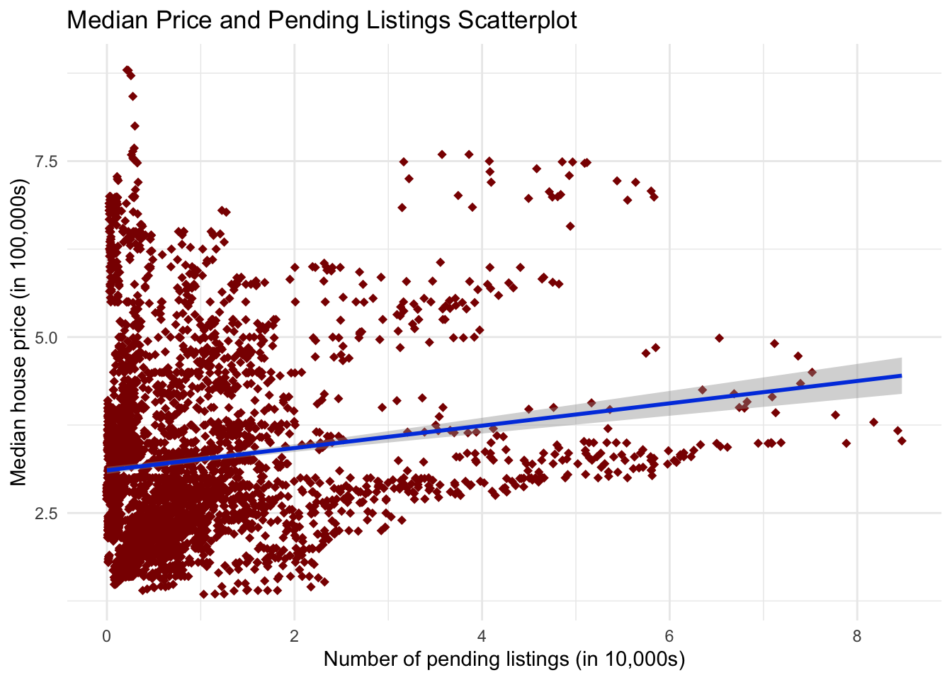
Comments on the First Graph
This graph shows the relationship between price and the number of pending listings. There could be a weak to moderate positive correlation based on the graph. This means the more pending listings, the higher the house price goes. This can only be confirmed with more testing.
2. Price and Days on Market Scatterplot
small.list %>%

     ggplot(aes(x = median_days_on_market,

                y = median_listing_price/100000)) +

     geom_point(color = "red4",

                shape = 18,

                size = 2) +

     stat_smooth(method = "lm", color = "#0245e0") +

     theme_minimal() +

     labs(x = "Median number of days on market",

          y = "Median house price (in 100,000s)") +

     ggtitle("Median Price and Median Days on Market Scatterplot")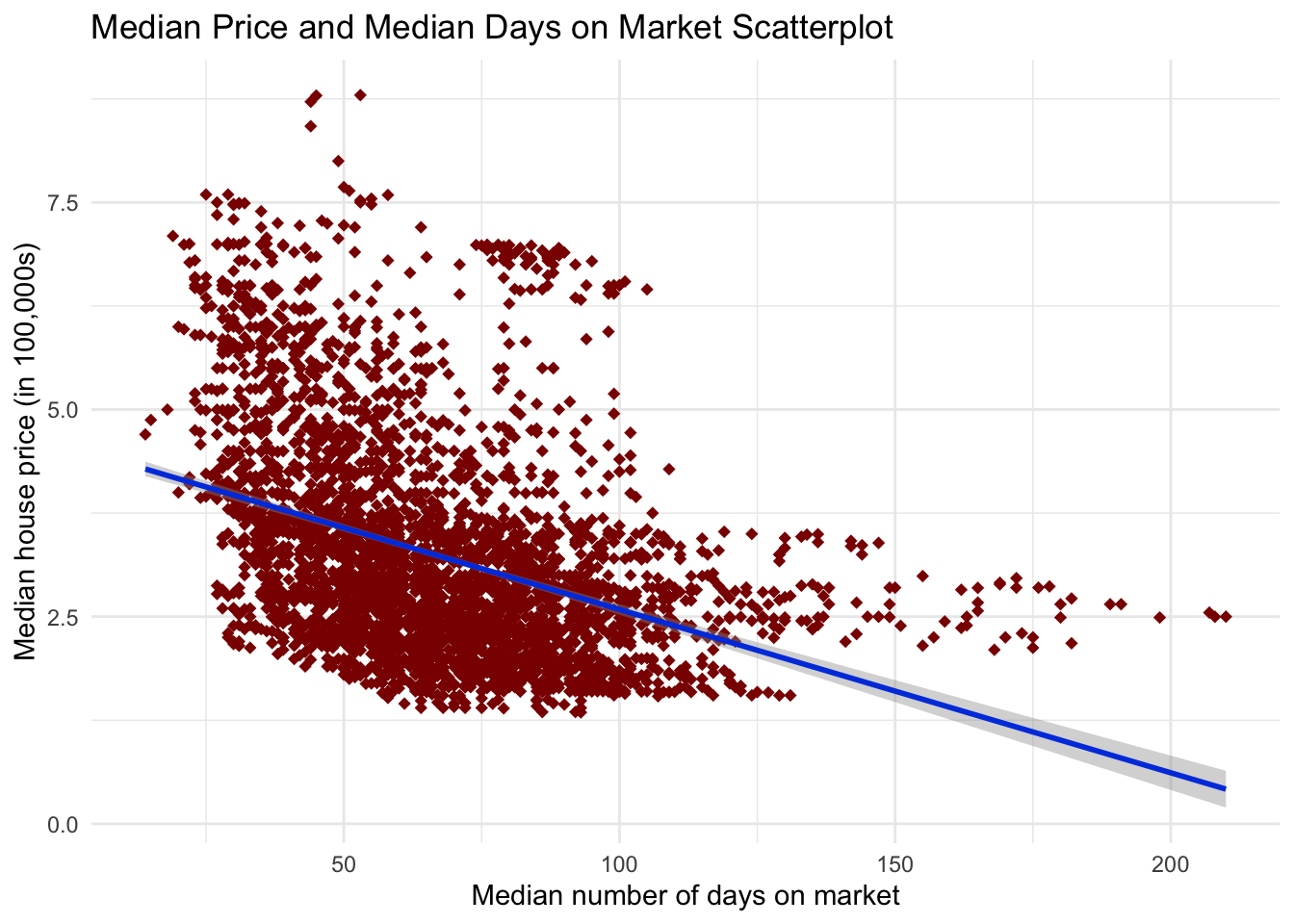
Comments on the Second Graph
This graph shows the relationship between price and the number of days on the market. There could be a moderate to strong negative correlation based on the graph. This means the more days on average houses are on the market, the lower the price of houses will go. This can only be confirmed with more testing.
3. Price and Season Boxplot
small.list %>%

     ggplot(aes(reorder(seasons, -median_listing_price/100000),

                median_listing_price/100000)) +

     geom_boxplot(aes(fill = seasons), show.legend = F) +

     scale_fill_manual(values = c("red", "blue", "green4", "purple")) +

     theme_minimal() +

     labs(x = "Seasons",

          y = "Median house price (in 100,000s)",

          fill = "Seasons") +

     ggtitle("Median Price and Seasons Boxplot")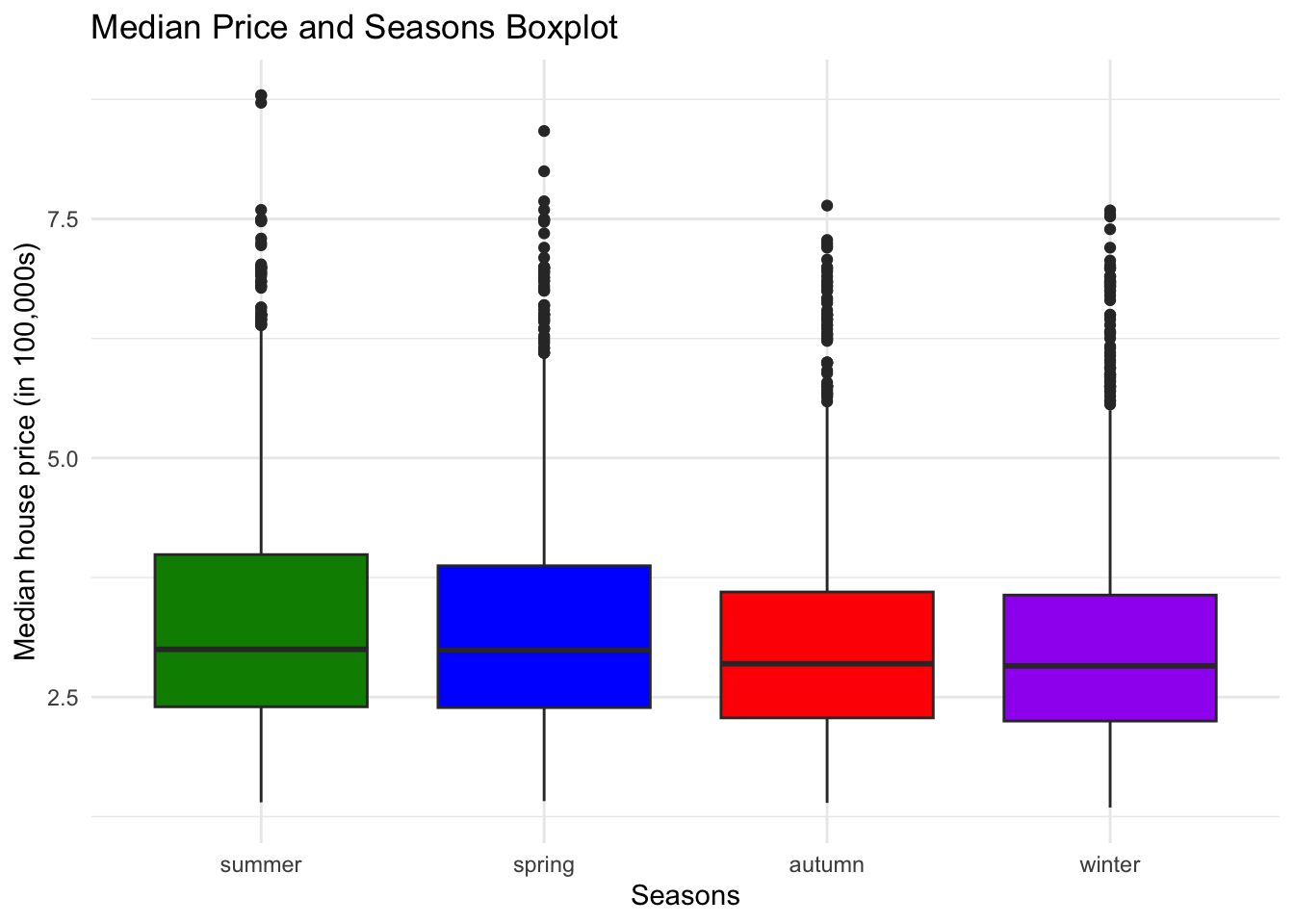
Comments on the Third Graph
This boxplot graph shows the relationship between price and the season of listing. This graph indicates marginal changes between seasons, but we can only know if this is significant through more testing. Also, of note, in the spring and summer, there are higher outliers in price, which could account for the differences we are seeing between seasons.
4. Price and Month Boxplot
small.list %>%

  ggplot(aes(x = month, y = median_listing_price/100000)) +

  geom_boxplot(aes(fill = month)) +

  scale_fill_brewer(palette = "Spectral") +

  theme_minimal() +

  labs(x = "Months",

       y = "Median house price (in 100,000s)") +

  scale_fill_discrete(name = "Months", labels = c("01 - Jan", "02 - Feb",

                                                  "03 - Mar", "04 - Apr",

                                                  "05 - May", "06 - Jun",

                                                  "07 - Jul", "08 - Aug",

                                                  "09 - Sep", "10 - Oct",

                                                  "11 - Nov", "12 - Dec")) +

     ggtitle("Median Price and Months Boxplot")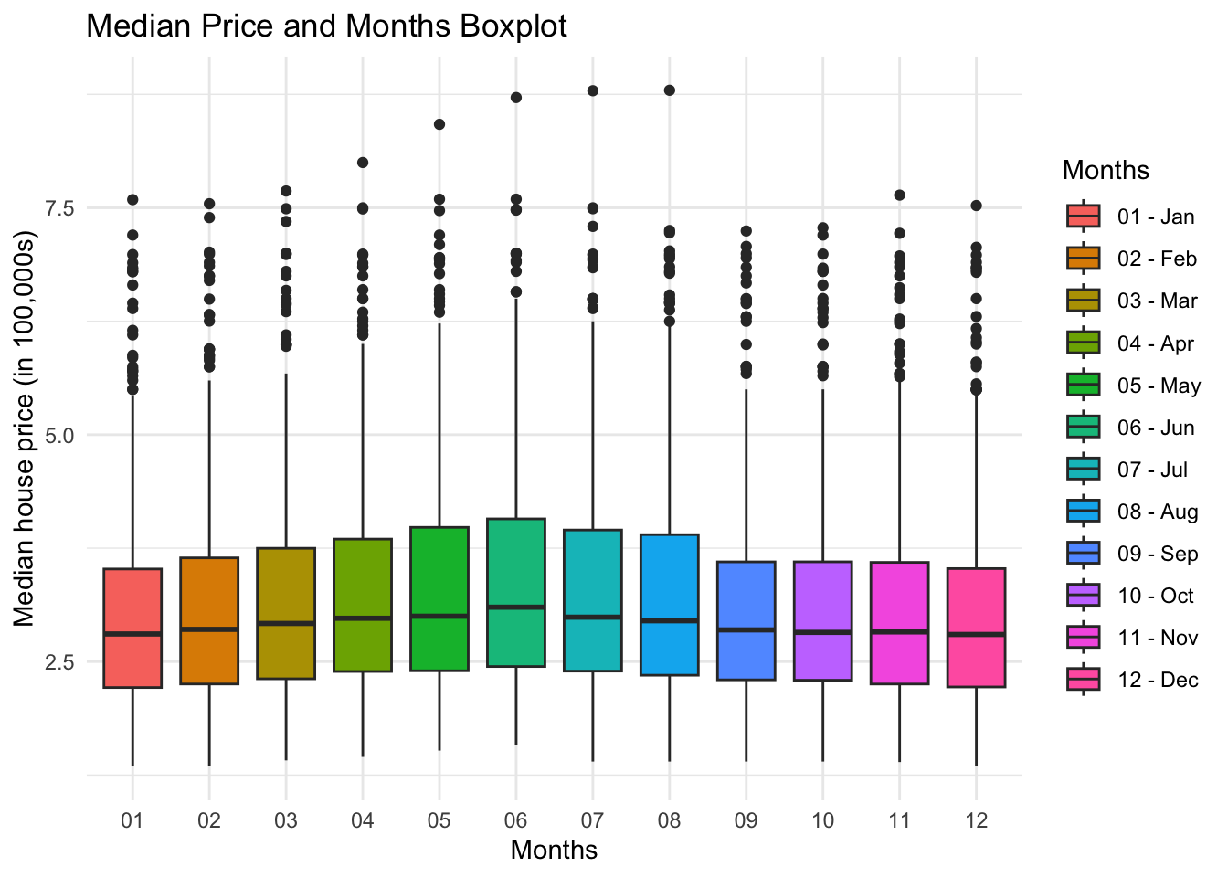
Comments on the Fourth Graph
This is a boxplot graph that shows the relationship between price and month. This information mirrors the previous boxplot with seasons: spring and summer have marginally higher prices. It is helpful to see which months are the highest and lowest with more granularity. It is also interesting to see that one outlier point for each month gets progressively higher in the summer months until the outliers drop off in September. This could account for the difference we are seeing seasonally.
5. Price and Region Boxplot
small.list %>%

  ggplot(aes(reorder(region, -median_listing_price/100000),

             median_listing_price/100000)) +

  geom_boxplot(aes(fill = region), show.legend = F) +

  scale_fill_manual(values = c("red", "blue", "green4",

                                    "purple", "orange")) +

  theme_minimal() +

  labs(x = "Regions in US",

       y = "Median house price (in 100,000s)") +

     ggtitle("Median Price and Regions Boxplot")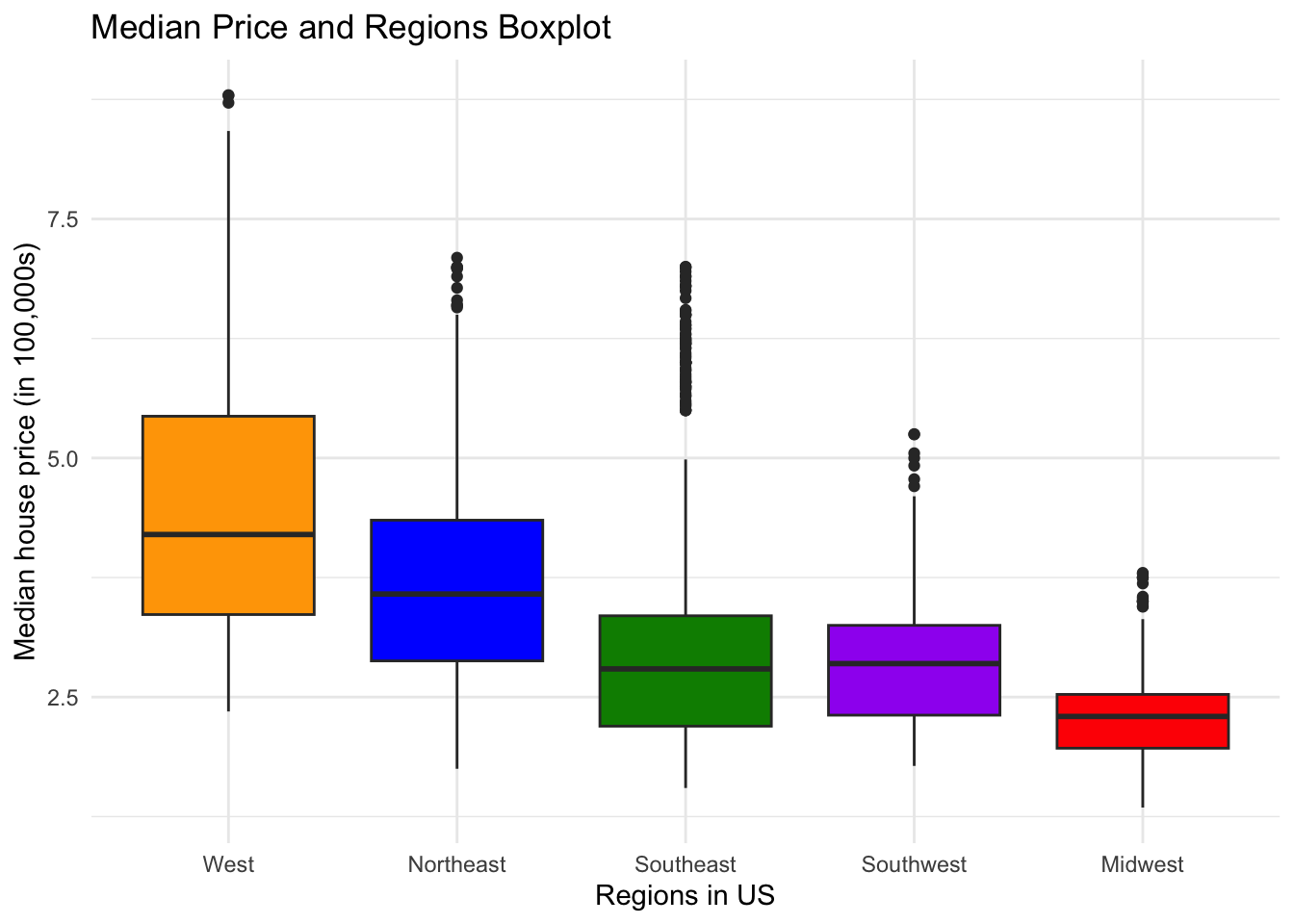
Comments on the Fifth Graph
This boxplot graph shows the relationship between the price and region of the listing. This indicates that there are substantial differences in price between regions, but we can only know if this is significant through more testing. The Western listings have the highest prices and the Midwest the lowest. Also, the Southeast listings have the most outliers in price.
6. Price and Year Boxplot
small.list %>%

     ggplot(aes(x = year, y = median_listing_price/100000)) +

     geom_boxplot(aes(fill = year)) +

     scale_fill_brewer(palette = "Spectral") +

     theme_minimal() +

          labs(x = "Year",

               y = "Median house price (in 100,000s)",

               fill = "Years") +

     ggtitle("Median Price and Years Boxplot")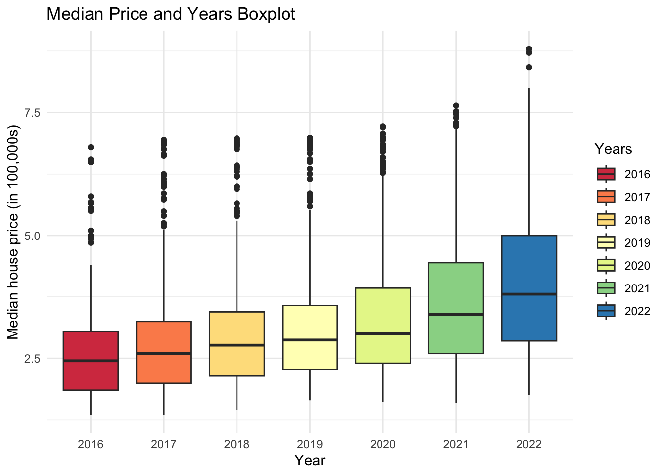
Comments on the Sixth Graph
This is a boxplot graph that shows the relationship between price and year. This indicates that there are notable differences in price over time. You can also see the steeper increase in price since 2020 (COVID).
7. Price and State Bar Chart (in order)
ggplot(small.list, aes(x = reorder(state_id, -median_listing_price/100000),

                       median_listing_price/100000)) +

  geom_bar(aes(fill = region), stat = "identity") +

  scale_x_discrete(guide = guide_axis(n.dodge = 2)) +

  labs(x = "States",

       y = "Median House Price (in 100,000s)",

       fill = "Regions (US)") +

  ggtitle("Median House Price by State") +

  theme_minimal()  +

  theme(legend.position = c(.55, 0.85),

        legend.direction = "horizontal")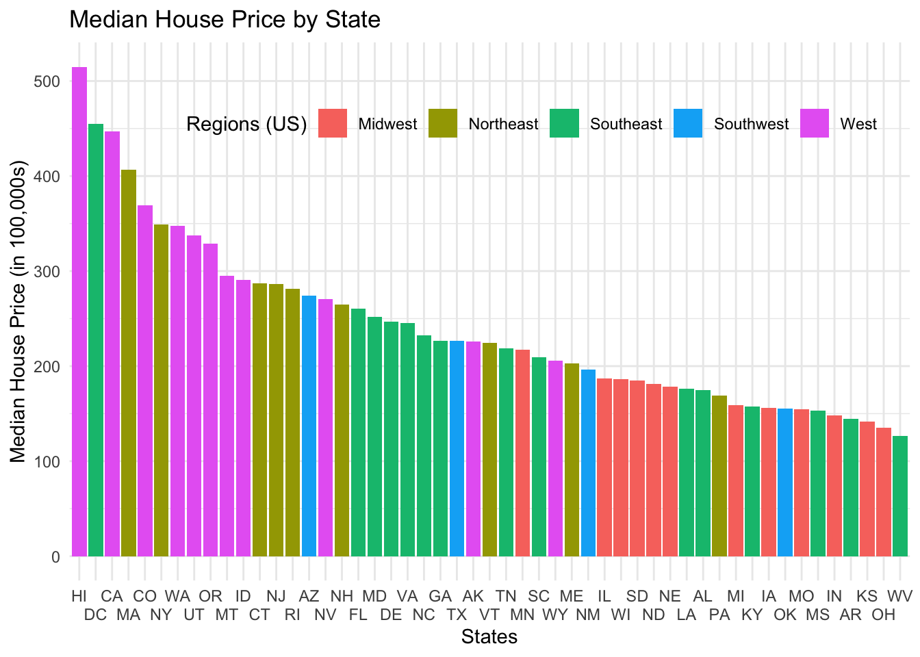
Comments on the Seventh Graph
This bar chart graph shows the relationship between the price and the state of the listing. This information mirrors the previous boxplot: the West has the highest prices, and the Midwest has the lowest. This is useful for seeing which states are highest and lowest with more granularity. Hawaii has the highest prices, while West Virginia has the lowest prices.
8. Price and State Scatterplot
ggerrorplot(small.list, x = "state_id",

            y = "median_listing_price/100000",

            desc_stat = "median_iqr",

            color = "black",

            add = "jitter",

            add.params = list(color = "lightblue2"),

            ggtheme = theme_minimal())  +

  scale_x_discrete(guide = guide_axis(n.dodge = 2))  +

  labs(x = "States",

       y = "Median House Price (in 100,000s)",

       fill = "Regions (US)") +

  ggtitle("Median House Price by State with Median point and IQR")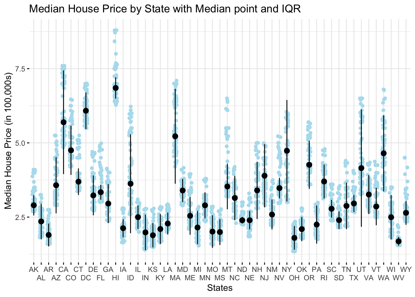
Comments on the Eighth Graph
This scatterplot graph shows the relationship between price and state of listing with the median and IQR shown. I wanted to show the upper and lower bounds of price by state and include the median and IQR. I found the package ggpubr helped to show it best. I wanted to show that because the bar chart helps see the upper limits, not the lower ones. When I tried to do a boxplot instead, it was too crowded to show much. Based on this graph, the state might be a huge indicator of a house’s price.
9. Price(Y) and Median Square Feet Scatterplot
small.list %>%

  ggplot(aes(x = median_square_feet,

             y = median_listing_price/100000)) +

  geom_point(color = "red4",

             shape = 18,

             size = 2) +

  stat_smooth(method = "lm", color = "#0245e0") +

  theme_minimal() +

  labs(x = "Median Sq Ft",

       y = "Median house price (in 100,000s)") +

     ggtitle("Median Price and Median Sq Ft Scatterplot")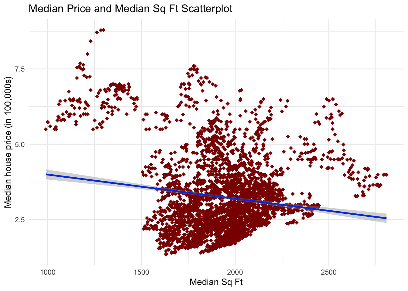
Comments on the Ninth Graph
This graph shows a weak negative relationship between Median sq ft and price; this might not make sense on the surface. This could be because of outliers or because there are so many different markets (essentially, the state the listing is in affects price more than sq ft).
10. Price(Y) and Active Listing Count Scatterplot
small.list %>%

  ggplot(aes(x = active_listing_count/10000,

             y = median_listing_price/100000)) +

  geom_point(color = "red4",

             shape = 18,

             size = 2) +

  stat_smooth(method = "lm", color = "#0245e0") +

  theme_minimal() +

  labs(x = "Number of active listings (in 10,000s)",

       y = "Median house price (in 100,000s)") +

     ggtitle("Median Price and Number of Active Listings Scatterplot")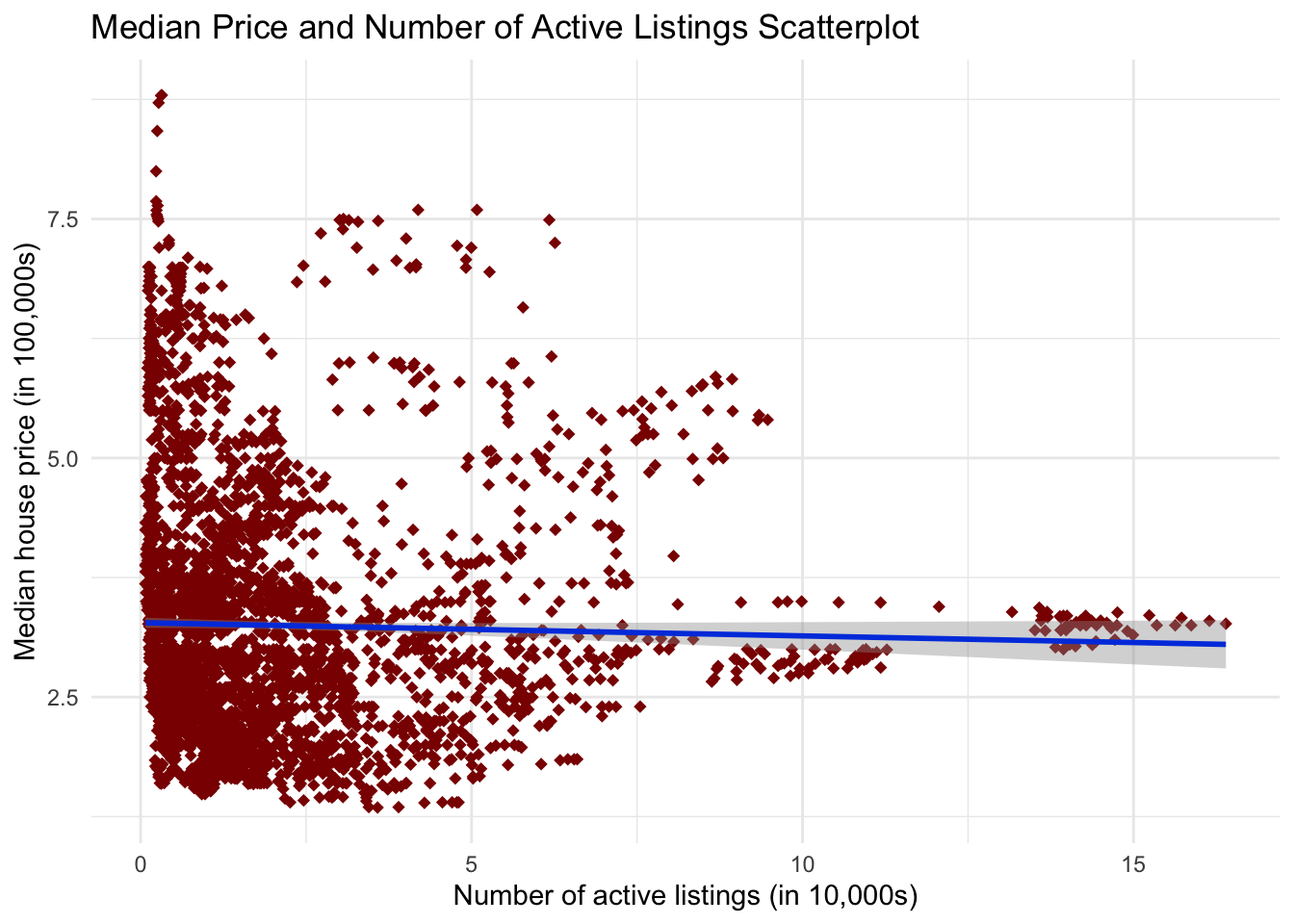
Comments on the Tenth Graph
This shows very little relationship between number of active listings and price.
11. Price(Y) and Monthly New Listing Count Scatterplot
small.list %>%

  ggplot(aes(x = monthly_new_listing_count/10000,

             y = median_listing_price/100000)) +

  geom_point(color = "red4",

             shape = 18,

             size = 2) +

  stat_smooth(method = "lm", color = "#0245e0") +

  theme_minimal() +

  labs(x = "Number of new monthly listings (in 10,000s)",

       y = "Median house price (in 100,000s)") +

     ggtitle("Median Price and Number of New Monthly Listings Scatterplot")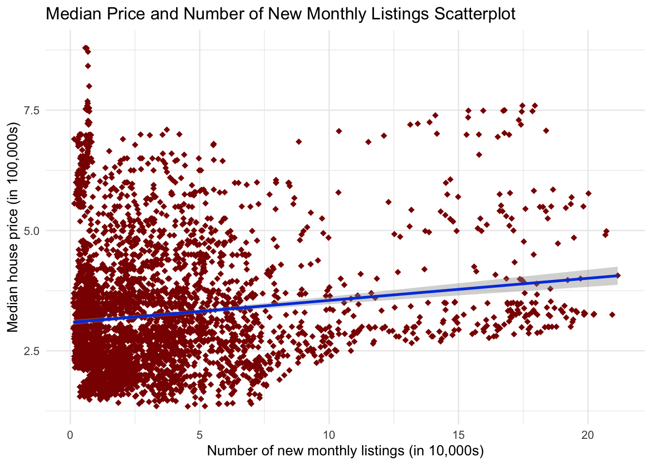
Comments on the Eleventh Graph
This shows a very weak positive relationship between price and the number of new monthly listings. This could be because the more new listings, the hotter the market is.
Step 5 - Predictions When Comparing Variables
Based on the graphs and statistics you choose from Steps 2-4, here are the predictions about what I may find when we compare the variables.
- Region affects housing prices.
- Based on the graph and other analyses, I think that region will affect price.
- This is also tied to the states variable.
- Season affects housing prices.
- There might be a marginal effect that season has on price. It likely will not have a huge impact, though.
- Pending Listings affect housing prices.
- I think the effect of the number of pending listings on price is marginal (weak positive). It likely will not have a huge impact, though.
- Days on the market affect housing prices.
- I think the effect of the number of days on the market on price is marginal (moderately negative).
- Time (what year it is) affects housing prices.
- What year it is might have a moderate to large effect on price.
- What state the listings are in affects housing prices.
- There might be a large effect on what state the listing is in on price.
- Median sq ft affects housing prices.
- Median sq ft may have a weak to moderate effect on price.
- Active listing count affects housing prices.
- The Active listing count may have a weak to moderate effect on price.
- Monthly new listing count affects housing prices.
- The Monthly new listing count may have a weak to moderate effect on price.
Step 6 - Hypothesis Testing
For this test, I will do multiple linear regression (with categorical variables), and the alpha is set to .05. I will adjust the variables based on the p-value approach.
Part 1: Set up the Null and Alternative Hypotheses
Hypothesis 1: Region affects housing prices.
H0: The slope of the line in regards to region is equal to zero.
HA: The slope of the line in regards to region is not equal to zero.
Hypothesis 2: Season affects housing prices.
H0: The slope of the line in regards to season is equal to zero.
HA: The slope of the line in regards to season is not equal to zero.
Hypothesis 3: The number of pending listings affects housing prices.
H0: The slope of the line in regard to the number of pending listings is equal to zero.
HA: The slope of the line in regard to the number of pending listings is not equal to zero.
Hypothesis 4: Days on the market affects housing prices.
H0: The slope of the line in regard to days on the market is equal to zero.
HA: The slope of the line in regard to days on the market is not equal to zero.
Hypothesis 5: Time (what year it is) affects housing prices.
H0: The slope of the line in regards to Time (what year it is) is equal to zero.
HA: The slope of the line in regards to Time (what year it is) is not equal to zero.
Hypothesis 6: What state the listings are in affects housing prices.
H0: The slope of the line in regards to states is equal to zero.
HA: The slope of the line in regards to states is not equal to zero.
Hypothesis 7: Median sq ft affects housing price.
H0: The slope of the line in regard to median sq ft is equal to zero.
HA: The slope of the line in regard to median sq ft is not equal to zero.
Hypothesis 8: Active listing count affects housing prices.
H0: The slope of the line in regard to the active listing count is equal to zero.
HA: The slope of the line in regard to the active listing count is not equal to zero.
Hypothesis 9: Monthly new listing count affects housing prices.
H0: The slope of the line in regard to the monthly new listing count is equal to zero.
HA: The slope of the line in regard to the monthly new listing count is not equal to zero.
Part 2 and 3: Compute the Test Statistic and Calculate the Probability
lm.small.list <- small.list %>%

  select(region, seasons, year, pending_listing_count,

         median_square_feet, monthly_new_listing_count,

         median_days_on_market, median_listing_price,

         active_listing_count, state)


lmStates <- lm(median_listing_price ~ ., data = lm.small.list)

summary(lmStates)
Call:
lm(formula = median_listing_price ~ ., data = lm.small.list)

Residuals:
    Min      1Q  Median      3Q     Max
-134476  -13717     800   12081  151439

Coefficients: (4 not defined because of singularities)
                            Estimate Std. Error t value Pr(>|t|)
(Intercept)                1.766e+05  1.556e+04  11.348  < 2e-16 ***
regionNortheast            7.843e+04  5.719e+03  13.712  < 2e-16 ***
regionSoutheast           -1.454e+04  4.985e+03  -2.917 0.003551 **
regionSouthwest           -1.704e+04  1.088e+04  -1.566 0.117463
regionWest                 3.258e+04  5.946e+03   5.478 4.58e-08 ***
seasonsspring             -5.771e+03  1.410e+03  -4.093 4.34e-05 ***
seasonssummer              7.494e+02  1.382e+03   0.542 0.587625
seasonswinter             -4.787e+03  1.617e+03  -2.960 0.003095 **
year2017                   1.476e+04  2.031e+03   7.267 4.47e-13 ***
year2018                   2.951e+04  2.080e+03  14.189  < 2e-16 ***
year2019                   4.199e+04  2.098e+03  20.017  < 2e-16 ***
year2020                   5.889e+04  2.227e+03  26.445  < 2e-16 ***
year2021                   8.138e+04  2.724e+03  29.873  < 2e-16 ***
year2022                   1.263e+05  2.965e+03  42.608  < 2e-16 ***
pending_listing_count      1.745e+00  1.753e-01   9.954  < 2e-16 ***
median_square_feet         2.725e+01  8.030e+00   3.394 0.000696 ***
monthly_new_listing_count -1.051e-01  6.493e-02  -1.618 0.105801
median_days_on_market     -4.561e+02  4.084e+01 -11.169  < 2e-16 ***
active_listing_count       5.614e-02  7.152e-02   0.785 0.432516
statealaska                3.385e+04  5.947e+03   5.692 1.35e-08 ***
statearizona               1.132e+05  9.612e+03  11.773  < 2e-16 ***
statearkansas             -3.757e+04  4.677e+03  -8.033 1.27e-15 ***
statecalifornia            2.611e+05  1.181e+04  22.112  < 2e-16 ***
statecolorado              1.896e+05  5.534e+03  34.266  < 2e-16 ***
stateconnecticut           5.773e+04  5.180e+03  11.144  < 2e-16 ***
statedelaware              1.047e+05  4.834e+03  21.663  < 2e-16 ***
statedistrict of columbia  3.876e+05  8.004e+03  48.429  < 2e-16 ***
stateflorida               3.523e+04  1.456e+04   2.419 0.015618 *
stategeorgia               1.791e+04  7.529e+03   2.378 0.017441 *
statehawaii                4.368e+05  8.348e+03  52.315  < 2e-16 ***
stateidaho                 9.923e+04  4.756e+03  20.865  < 2e-16 ***
stateillinois             -3.005e+04  6.097e+03  -4.929 8.64e-07 ***
stateindiana              -5.896e+04  4.754e+03 -12.401  < 2e-16 ***
stateiowa                 -3.608e+04  4.820e+03  -7.486 8.83e-14 ***
statekansas               -6.166e+04  4.969e+03 -12.408  < 2e-16 ***
statekentucky             -2.970e+04  4.705e+03  -6.312 3.08e-10 ***
statelouisiana             2.272e+03  4.648e+03   0.489 0.624969
statemaine                -3.115e+04  5.293e+03  -5.885 4.33e-09 ***
statemaryland              9.564e+04  4.839e+03  19.762  < 2e-16 ***
statemassachusetts         2.171e+05  5.648e+03  38.445  < 2e-16 ***
statemichigan             -3.474e+04  5.009e+03  -6.936 4.75e-12 ***
stateminnesota             2.482e+04  4.977e+03   4.987 6.41e-07 ***
statemississippi          -2.411e+04  4.721e+03  -5.107 3.44e-07 ***
statemissouri             -4.880e+04  4.614e+03 -10.577  < 2e-16 ***
statemontana               1.203e+05  4.613e+03  26.087  < 2e-16 ***
statenebraska             -1.698e+04  5.059e+03  -3.357 0.000796 ***
statenevada                7.238e+04  5.302e+03  13.652  < 2e-16 ***
statenew hampshire         2.872e+04  5.103e+03   5.628 1.96e-08 ***
statenew jersey            5.175e+04  6.660e+03   7.770 1.01e-14 ***
statenew mexico            3.584e+04  1.187e+04   3.019 0.002554 **
statenew york              1.256e+05  8.054e+03  15.598  < 2e-16 ***
statenorth carolina        5.263e+04  5.586e+03   9.423  < 2e-16 ***
statenorth dakota         -4.728e+03  5.700e+03  -0.829 0.406946
stateohio                 -9.101e+04  5.153e+03 -17.660  < 2e-16 ***
stateoklahoma             -2.741e+04  1.134e+04  -2.418 0.015674 *
stateoregon                1.520e+05  5.241e+03  28.997  < 2e-16 ***
statepennsylvania         -1.125e+05  6.807e+03 -16.531  < 2e-16 ***
staterhode island          5.345e+04  6.218e+03   8.595  < 2e-16 ***
statesouth carolina        3.338e+04  4.780e+03   6.984 3.40e-12 ***
statesouth dakota         -2.547e+03  5.189e+03  -0.491 0.623600
statetennessee             3.830e+04  4.854e+03   7.890 3.95e-15 ***
statetexas                        NA         NA      NA       NA
stateutah                  1.390e+05  6.097e+03  22.797  < 2e-16 ***
statevermont                      NA         NA      NA       NA
statevirginia              7.668e+04  4.950e+03  15.491  < 2e-16 ***
statewashington            1.644e+05  5.527e+03  29.743  < 2e-16 ***
statewest virginia        -4.987e+04  5.073e+03  -9.831  < 2e-16 ***
statewisconsin                    NA         NA      NA       NA
statewyoming                      NA         NA      NA       NA
---
Signif. codes:  0 '***' 0.001 '**' 0.01 '*' 0.05 '.' 0.1 ' ' 1

Residual standard error: 27890 on 3689 degrees of freedom
  (20 observations deleted due to missingness)
Multiple R-squared:  0.9549,    Adjusted R-squared:  0.9542
F-statistic:  1222 on 64 and 3689 DF,  p-value: < 2.2e-16
The adjusted r-squared is 0.9542, which is very strong.
Next, we need to start removing variables based on the highest p-value while checking the adjusted r-squared to ensure we are not removing something important.
Since there are categorical variables, we do need to worry about one being significant based on it being a category of another significant variable. In this case, the highest is the active_listing_count variable, with a p-value of 0.432516.
lmStates <- lm(median_listing_price ~ . - active_listing_count,

               data = lm.small.list)

summary(lmStates)
Call:
lm(formula = median_listing_price ~ . - active_listing_count,
    data = lm.small.list)

Residuals:
    Min      1Q  Median      3Q     Max
-133857  -13637     770   12067  151752

Coefficients: (4 not defined because of singularities)
                            Estimate Std. Error t value Pr(>|t|)
(Intercept)                1.765e+05  1.556e+04  11.341  < 2e-16 ***
regionNortheast            7.726e+04  5.524e+03  13.987  < 2e-16 ***
regionSoutheast           -1.483e+04  4.971e+03  -2.985 0.002859 **
regionSouthwest           -1.310e+04  9.657e+03  -1.357 0.174919
regionWest                 3.133e+04  5.730e+03   5.468 4.86e-08 ***
seasonsspring             -5.929e+03  1.395e+03  -4.249 2.20e-05 ***
seasonssummer              7.411e+02  1.382e+03   0.536 0.591718
seasonswinter             -4.993e+03  1.595e+03  -3.129 0.001766 **
year2017                   1.459e+04  2.020e+03   7.225 6.08e-13 ***
year2018                   2.929e+04  2.062e+03  14.209  < 2e-16 ***
year2019                   4.181e+04  2.085e+03  20.053  < 2e-16 ***
year2020                   5.857e+04  2.189e+03  26.752  < 2e-16 ***
year2021                   8.089e+04  2.652e+03  30.496  < 2e-16 ***
year2022                   1.257e+05  2.865e+03  43.888  < 2e-16 ***
pending_listing_count      1.672e+00  1.488e-01  11.240  < 2e-16 ***
median_square_feet         2.801e+01  7.972e+00   3.513 0.000448 ***
monthly_new_listing_count -8.861e-02  6.146e-02  -1.442 0.149471
median_days_on_market     -4.526e+02  4.060e+01 -11.150  < 2e-16 ***
statealaska                3.416e+04  5.934e+03   5.757 9.27e-09 ***
statearizona               1.093e+05  8.244e+03  13.257  < 2e-16 ***
statearkansas             -3.780e+04  4.667e+03  -8.101 7.36e-16 ***
statecalifornia            2.651e+05  1.064e+04  24.916  < 2e-16 ***
statecolorado              1.905e+05  5.421e+03  35.143  < 2e-16 ***
stateconnecticut           5.846e+04  5.097e+03  11.468  < 2e-16 ***
statedelaware              1.039e+05  4.734e+03  21.959  < 2e-16 ***
statedistrict of columbia  3.874e+05  7.999e+03  48.433  < 2e-16 ***
stateflorida               4.241e+04  1.133e+04   3.743 0.000185 ***
stategeorgia               2.012e+04  6.979e+03   2.884 0.003951 **
statehawaii                4.375e+05  8.286e+03  52.808  < 2e-16 ***
stateidaho                 9.950e+04  4.743e+03  20.979  < 2e-16 ***
stateillinois             -2.826e+04  5.654e+03  -4.998 6.06e-07 ***
stateindiana              -5.926e+04  4.738e+03 -12.507  < 2e-16 ***
stateiowa                 -3.631e+04  4.811e+03  -7.548 5.52e-14 ***
statekansas               -6.241e+04  4.876e+03 -12.801  < 2e-16 ***
statekentucky             -2.973e+04  4.704e+03  -6.320 2.93e-10 ***
statelouisiana             2.242e+03  4.648e+03   0.482 0.629661
statemaine                -3.075e+04  5.268e+03  -5.837 5.77e-09 ***
statemaryland              9.569e+04  4.839e+03  19.776  < 2e-16 ***
statemassachusetts         2.177e+05  5.596e+03  38.911  < 2e-16 ***
statemichigan             -3.433e+04  4.982e+03  -6.892 6.45e-12 ***
stateminnesota             2.473e+04  4.976e+03   4.970 7.02e-07 ***
statemississippi          -2.459e+04  4.681e+03  -5.254 1.57e-07 ***
statemissouri             -4.862e+04  4.608e+03 -10.551  < 2e-16 ***
statemontana               1.205e+05  4.608e+03  26.144  < 2e-16 ***
statenebraska             -1.783e+04  4.942e+03  -3.608 0.000313 ***
statenevada                7.299e+04  5.245e+03  13.914  < 2e-16 ***
statenew hampshire         2.897e+04  5.092e+03   5.689 1.37e-08 ***
statenew jersey            5.359e+04  6.234e+03   8.596  < 2e-16 ***
statenew mexico            3.108e+04  1.021e+04   3.045 0.002342 **
statenew york              1.292e+05  6.635e+03  19.473  < 2e-16 ***
statenorth carolina        5.399e+04  5.309e+03  10.171  < 2e-16 ***
statenorth dakota         -5.915e+03  5.495e+03  -1.076 0.281819
stateohio                 -9.014e+04  5.033e+03 -17.910  < 2e-16 ***
stateoklahoma             -3.180e+04  9.861e+03  -3.225 0.001272 **
stateoregon                1.527e+05  5.155e+03  29.625  < 2e-16 ***
statepennsylvania         -1.102e+05  6.142e+03 -17.946  < 2e-16 ***
staterhode island          5.390e+04  6.190e+03   8.708  < 2e-16 ***
statesouth carolina        3.399e+04  4.715e+03   7.210 6.78e-13 ***
statesouth dakota         -3.563e+03  5.024e+03  -0.709 0.478218
statetennessee             3.867e+04  4.830e+03   8.007 1.56e-15 ***
statetexas                        NA         NA      NA       NA
stateutah                  1.393e+05  6.082e+03  22.907  < 2e-16 ***
statevermont                      NA         NA      NA       NA
statevirginia              7.733e+04  4.881e+03  15.843  < 2e-16 ***
statewashington            1.653e+05  5.406e+03  30.575  < 2e-16 ***
statewest virginia        -5.033e+04  5.038e+03  -9.989  < 2e-16 ***
statewisconsin                    NA         NA      NA       NA
statewyoming                      NA         NA      NA       NA
---
Signif. codes:  0 '***' 0.001 '**' 0.01 '*' 0.05 '.' 0.1 ' ' 1

Residual standard error: 27890 on 3690 degrees of freedom
  (20 observations deleted due to missingness)
Multiple R-squared:  0.9549,    Adjusted R-squared:  0.9542
F-statistic:  1241 on 63 and 3690 DF,  p-value: < 2.2e-16
The adjusted r-squared is 0.9542, which is the same after removing active_listing_count. This tells us we are on the right track.
We still have insignificant variables, so we want to do that again. The next variable to remove is monthly_new_listing_count, with a p-value of 0.149471.
lmStates <- lm(median_listing_price ~ .

               - active_listing_count - monthly_new_listing_count,

               data = lm.small.list)

summary(lmStates)
Call:
lm(formula = median_listing_price ~ . - active_listing_count -
    monthly_new_listing_count, data = lm.small.list)

Residuals:
    Min      1Q  Median      3Q     Max
-134706  -13727     790   12145  151922

Coefficients: (4 not defined because of singularities)
                            Estimate Std. Error t value Pr(>|t|)
(Intercept)                1.759e+05  1.556e+04  11.303  < 2e-16 ***
regionNortheast            7.897e+04  5.396e+03  14.636  < 2e-16 ***
regionSoutheast           -1.462e+04  4.969e+03  -2.942 0.003281 **
regionSouthwest           -2.124e+04  7.835e+03  -2.712 0.006728 **
regionWest                 3.333e+04  5.560e+03   5.994 2.24e-09 ***
seasonsspring             -6.388e+03  1.359e+03  -4.702 2.67e-06 ***
seasonssummer              2.694e+02  1.343e+03   0.201 0.840986
seasonswinter             -4.713e+03  1.584e+03  -2.976 0.002942 **
year2017                   1.435e+04  2.013e+03   7.129 1.21e-12 ***
year2018                   2.900e+04  2.052e+03  14.133  < 2e-16 ***
year2019                   4.160e+04  2.080e+03  19.998  < 2e-16 ***
year2020                   5.879e+04  2.184e+03  26.915  < 2e-16 ***
year2021                   8.117e+04  2.646e+03  30.676  < 2e-16 ***
year2022                   1.260e+05  2.861e+03  44.029  < 2e-16 ***
pending_listing_count      1.604e+00  1.410e-01  11.375  < 2e-16 ***
median_square_feet         2.713e+01  7.950e+00   3.413 0.000650 ***
median_days_on_market     -4.475e+02  4.045e+01 -11.064  < 2e-16 ***
statealaska                3.373e+04  5.927e+03   5.691 1.36e-08 ***
statearizona               1.165e+05  6.575e+03  17.711  < 2e-16 ***
statearkansas             -3.707e+04  4.640e+03  -7.990 1.79e-15 ***
statecalifornia            2.543e+05  7.577e+03  33.569  < 2e-16 ***
statecolorado              1.880e+05  5.126e+03  36.670  < 2e-16 ***
stateconnecticut           5.737e+04  5.042e+03  11.378  < 2e-16 ***
statedelaware              1.055e+05  4.613e+03  22.865  < 2e-16 ***
statedistrict of columbia  3.886e+05  7.957e+03  48.837  < 2e-16 ***
stateflorida               3.270e+04  9.117e+03   3.587 0.000339 ***
stategeorgia               1.572e+04  6.274e+03   2.505 0.012284 *
statehawaii                4.366e+05  8.261e+03  52.851  < 2e-16 ***
stateidaho                 9.893e+04  4.727e+03  20.929  < 2e-16 ***
stateillinois             -3.163e+04  5.150e+03  -6.141 9.06e-10 ***
stateindiana              -5.944e+04  4.737e+03 -12.546  < 2e-16 ***
stateiowa                 -3.560e+04  4.786e+03  -7.438 1.26e-13 ***
statekansas               -6.126e+04  4.810e+03 -12.735  < 2e-16 ***
statekentucky             -2.917e+04  4.689e+03  -6.221 5.49e-10 ***
statelouisiana             2.785e+03  4.633e+03   0.601 0.547764
statemaine                -3.127e+04  5.257e+03  -5.949 2.95e-09 ***
statemaryland              9.522e+04  4.828e+03  19.721  < 2e-16 ***
statemassachusetts         2.157e+05  5.414e+03  39.840  < 2e-16 ***
statemichigan             -3.659e+04  4.729e+03  -7.737 1.30e-14 ***
stateminnesota             2.477e+04  4.976e+03   4.977 6.74e-07 ***
statemississippi          -2.339e+04  4.606e+03  -5.077 4.02e-07 ***
statemissouri             -4.894e+04  4.603e+03 -10.633  < 2e-16 ***
statemontana               1.203e+05  4.607e+03  26.109  < 2e-16 ***
statenebraska             -1.623e+04  4.816e+03  -3.370 0.000760 ***
statenevada                7.179e+04  5.180e+03  13.859  < 2e-16 ***
statenew hampshire         2.889e+04  5.092e+03   5.673 1.51e-08 ***
statenew jersey            4.945e+04  5.534e+03   8.935  < 2e-16 ***
statenew mexico            4.064e+04  7.760e+03   5.238 1.71e-07 ***
statenew york              1.247e+05  5.853e+03  21.304  < 2e-16 ***
statenorth carolina        5.203e+04  5.132e+03  10.139  < 2e-16 ***
statenorth dakota         -3.908e+03  5.317e+03  -0.735 0.462335
stateohio                 -9.198e+04  4.869e+03 -18.890  < 2e-16 ***
stateoklahoma             -2.298e+04  7.735e+03  -2.971 0.002989 **
stateoregon                1.511e+05  5.028e+03  30.047  < 2e-16 ***
statepennsylvania         -1.139e+05  5.573e+03 -20.445  < 2e-16 ***
staterhode island          5.380e+04  6.191e+03   8.690  < 2e-16 ***
statesouth carolina        3.362e+04  4.709e+03   7.140 1.12e-12 ***
statesouth dakota         -1.685e+03  4.853e+03  -0.347 0.728437
statetennessee             3.777e+04  4.790e+03   7.886 4.09e-15 ***
statetexas                        NA         NA      NA       NA
stateutah                  1.388e+05  6.074e+03  22.859  < 2e-16 ***
statevermont                      NA         NA      NA       NA
statevirginia              7.569e+04  4.748e+03  15.943  < 2e-16 ***
statewashington            1.629e+05  5.141e+03  31.683  < 2e-16 ***
statewest virginia        -4.911e+04  4.967e+03  -9.886  < 2e-16 ***
statewisconsin                    NA         NA      NA       NA
statewyoming                      NA         NA      NA       NA
---
Signif. codes:  0 '***' 0.001 '**' 0.01 '*' 0.05 '.' 0.1 ' ' 1

Residual standard error: 27890 on 3691 degrees of freedom
  (20 observations deleted due to missingness)
Multiple R-squared:  0.9549,    Adjusted R-squared:  0.9542
F-statistic:  1261 on 62 and 3691 DF,  p-value: < 2.2e-16
The adjusted r-squared is 0.9542, which is the same after removing monthly_new_listing_count. We removed all the insignificant p-values that were left that were not categorical values tied to significant values. Therefore, this should be the final model.
Parts 4 and 5: Interpret the Probability and Write a Conclusion
As I mentioned earlier, the adjusted r-squared is 0.9542, which is a strong model.
We see an overall F-statistic in our output with a p-value of < 2.2e-16, which is less than .05. This indicates that our overall model is significant.
Hypotheses
Hypothesis 1: Region affects housing prices.
The output shows a p-value on the region rows < .001 from a t-test, which is significant. This significance means our predictor variable influences the Y variable and that we can reject the null hypothesis and support our alternative hypothesis.
Hypothesis 2: Season affects housing prices.
The output shows a p-value on the season rows < .001 from a t-test, which is significant. This significance means our predictor variable influences the Y variable and that we can reject the null hypothesis and support our alternative hypothesis.
Hypothesis 3: The number of pending listings affects housing prices.
The output shows a p-value on the pending listings row < 2e-16 from a t-test, which is significant. This significance means our predictor variable influences the Y variable and that we can reject the null hypothesis and support our alternative hypothesis.
Hypothesis 4: Days on the market affects housing prices.
The output shows a p-value on the Days on market row < 2e-16 from a t-test, which is significant. This significance means our predictor variable influences the Y variable and that we can reject the null hypothesis and support our alternative hypothesis.
Hypothesis 5: Time (what year it is) affects housing prices.
The output shows a p-value on the year rows < .001 from a t-test, which is significant. This significance means our predictor variable influences the Y variable and that we can reject the null hypothesis and support our alternative hypothesis.
Hypothesis 6: What state the listings are in affects housing prices.
The output shows a p-value on the state rows < .001 from a t-test, which is significant. This significance means our predictor variable influences the Y variable and that we can reject the null hypothesis and support our alternative hypothesis.
Hypothesis 7: Median sq ft affects housing price.
The output shows a p-value on the Median sq ft row 0.000650 from a t-test, which is significant. This significance means our predictor variable influences the Y variable and that we can reject the null hypothesis and support our alternative hypothesis.
Hypothesis 8: Active listing count affects housing prices.
The output shows a p-value on the Active listing count row of 0.432516 from a t-value. This is NOT significant at any appropriate level of alpha. This lack of significance means our predictor variable does NOT influence the Y variable, and we fail to reject the null hypothesis that there is a slope.
Hypothesis 9: Monthly new listing count affects housing prices.
The output shows a p-value on the Monthly new listing count row of 0.149471 from a t-value. This is NOT significant at any appropriate level of alpha. This lack of significance means our predictor variable does NOT influence the Y variable, and we fail to reject the null hypothesis that there is a slope.
Our final model finds that the region, seasons, year, pending_listing_count, median_square_feet, median_days_on_market, and which state the listing is are the best predictors of housing price. We also find that the price goes down the more days on the market. Pending_listing_count, median_square_feet, and years as time goes on all had positive relationships with price, so the higher any of those categories are, the higher the housing price will be. These factors explain about 95.42% of the variance in price, which is a strong model.
Evaluating My Predictions
I was mostly correct in my predictions. I thought that active and new listings would have had a more substantial impact on the model and not been statistically insignificant (other than active listings). I also thought that median sq ft had a weaker relationship with price based on the graph.
Step 7 - Final Thoughts
As I mentioned earlier, we find that the region, seasons, year, pending_listing_count, median_square_feet, median_days_on_market, and which state the listing is in are the best predictors of housing price.
One of the greatest factors that could affect the results is that much of the data was very heavily skewed, and most of the tests require the data to be normally distributed. Also, the data in certain circumstances might not be linear. Other factors that could affect the results are outliers in the data that can distort the results a bit. Also, there are potentially lurking variables not accounted for in this data set that we could not add to the model that would have made an impact. Examples of lurking variables could be the number of buyers in the market, the number of bidders per house, the difference in listing price vs. sold price, the population of the region, the socioeconomic status of the region, crime rates, the number of schools, house taxes, taxes in general, etc.
Also, some biases could affect our results as well. For certain variables, it is unclear if it affects price or price affects it first–such as median days available on the market. The price may make it take longer to sell in the first place rather than the fact that it is taking longer to sell houses in that market, prompting people to make their house prices lower in the first place.
Finally, of course, there are limitations to my knowledge. Since I am still new at this, there may have been circumstances where there are better tests to perform, transformations of data, better ways to group the data, or better variables to pick at the outset. As I continue to learn more, I hope to gain better strategies for analysis.
Comments on by State Grouping
The most expensive places are in the West and Northeast. For Hawaii and DC, it might also be about scarcity–they seem like outliers for median active, median pending, and new listings. The West and South (mainly Southeast, but Texas as well) have the largest homes for sale on average. Vermont and Maine seem like outliers for the Northeast on median days on the market. Otherwise, the homes on the eastern side (Northeast and Southeast) generally have the highest median days on the market. The West has the least days on the market on average. These comments are based on the top 10, so I will only know for sure if further analysis is done.