Coding Demo of how to optimize a mobile robot's path in a warehouse environment with reinforcement learning

The Goal

Let's consider a mobile robot in a warehouse environment that is used to retrieve items in the warehouse for packing. We want to give the robot a location of the desired item(s) and the starting place of the robot, and the robot should be able to figure out the shortest path to go and retrieve the objects. The robot must avoid obstacles in its path, or it will get a negative reward if it runs into it. To incentivize the robot to move to the desired location(s) as quickly as possible, there is also a slight negative reward for every step it takes.

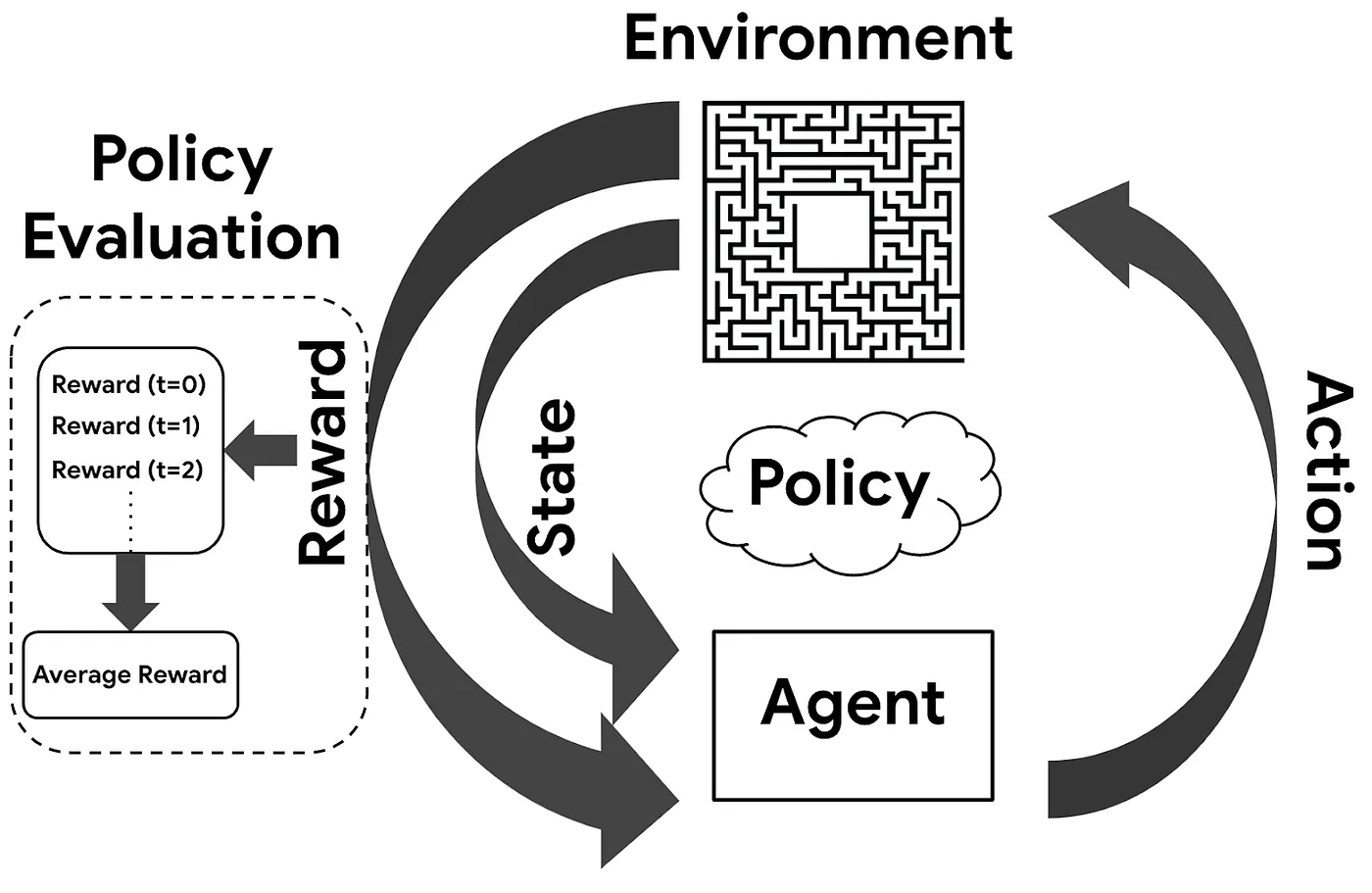
As we move through this demo, it is important to remember the overall Reinforcement Learning process we use to train this robot. The diagram below shows the overall process for how Reinforcement Learning works.

Image Source: https://blog.research.google/2020/04/off-policy-estimation-for-infinite.html

Note–this type of path planning can also be used in other ways. For instance, in the presentation, we also talk about how this same method could be used to optimize the path of a package in a warehouse to a truck to be shipped.

Why would you use Reinforcement Learning?

Here are some of the reasons:

• The robot does not need to be explicitly told what paths are best.

• The Q-Learning Algorithm can be re-trained relatively easily with a new environment configuration (different obstacles, etc.).

• Reinforcement Learning can continually optimize as time goes on.

• Businesses would not necessarily need to rely on complicated and cumbersome automation strategies to do the same task.

Here are some of the downsides:

• By its nature, Reinforcement Learning is not guaranteed to find the optimal solution every time. However, it is likely that it will at least get close, and it is far faster and simpler compared to a full optimization problem.

Import Libraries and Set Seed

# Importing Numpy Library
import numpy as np

# Turn legacy formatting ON
np.set_printoptions(legacy='1.13')

# Setting seed for reproducibility
np.random.seed(1693)

Understanding the Environment -- Warehouse Layout Visual

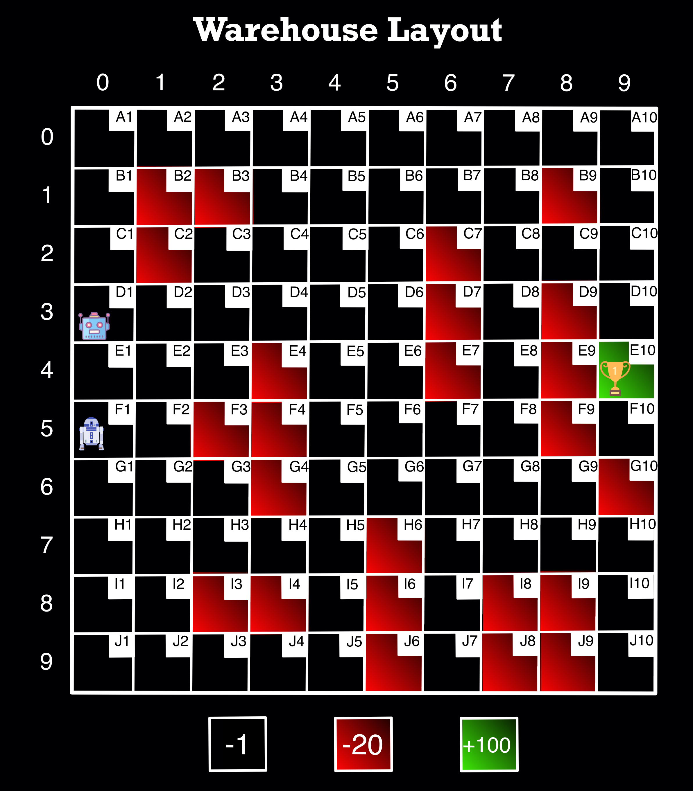
Image Source: Author

• The entire environment is comprised of 100 squares with 10 rows and 10 columns.

• The indices of the rows and columns start at 0—so they are indexed as 0 through 9 (as shown on the top and left of the image). We use the indices when going through the loops to determine our states later.

• For user ease, every cell in the environment has a code name in the top right corner of each cell (example: A1, J10, etc.)

• There are two robots in the diagram, and for this demo, the “user” would just choose which one to use based on its starting location.

• The cells highlighted in red are obstacles that the robot cannot traverse and are given a penalty of -20, as shown at the bottom of the image.

• In the environment, one or more cells may be highlighted in green, representing the goal(s) the robot is trying to reach. When the robot reaches the goal, it is given a reward of +100, as shown at the bottom of the image.

• Finally, the black—or empty—cells represent the possible cells the robot can choose as part of the path that it is allowed to move along. They have values of -1 to motivate the robot to hurry up (and generate the shortest path).

Initial Setup and Defining Functions Part 1

# This represents the environment rewards in an array
rewardList = [
[-1.,   -1.,   -1.,   -1.,   -1.,   -1.,   -1.,   -1.,  -1.,  -1.],
[-1.,   -20.,  -20.,  -1.,   -1.,   -1.,   -1.,   -1.,  -20., -1.],
[-1.,   -20.,  -1.,   -1.,   -1.,   -1.,   -20.,  -1.,  -1.,  -1.],
[-1.,   -1.,   -1.,   -1.,   -1.,   -1.,   -20.,  -1.,  -20., -1.],
[-1.,   -1.,   -1.,   -20.,  -1.,   -1.,   -20.,  -1.,  -20., -1.],
[-1.,   -1.,   -20.,  -20.,  -1.,   -1.,   -1.,   -1.,  -20., -1.],
[-1.,   -1.,   -1.,   -20.,  -1.,   -1.,   -1.,   -1.,  -1.,  -20.],
[-1.,   -1.,   -1.,   -1.,   -1.,   -20.,  -1.,   -1.,  -1.,  -1.],
[-1.,   -1.,   -20.,  -20.,  -1.,   -20.,  -1.,   -20., -20., -1.],
[-1.,   -1.,   -1.,   -1.,   -1.,   -20.,  -1.,   -20., -20., -1.]
]
map_rewards=np.array(rewardList)

Note -- When we set up the initial array map_rewards, we do not include the goal location(s) so we can train our model to go anywhere in the environment.

# Create variables needed later
actions = ['up', 'right', 'down', 'left'] # Possible actions the robot can take
WHrows = 10     # warehouse rows
WHcols = 10     # warehouse columns

# Creates a dictionary with a code name for every pair of indices for every grid cell
# The indices are given in tuples as the key and the codename as the value

keys = []

for i in range(0,10):
  for j in range(0,10):
    keys.append((i,j))

values = []

for v in ["A","B","C","D","E","F","G","H","I","J"]:
  for k in range(1,11):
    value = v + str(k)
    values.append(value)

codeNames = dict(zip(keys, values))

# This function finds a random legal row and column to start on while training

# Important to have a variety of starting places so we do not only train our model
# to start from one place -- we want to be able to start from anywhere

def start_pos():
    """
    Select starting legal position for each episode randomly

    Args:

    returns:
          row(int): index of row of start position of robot
          col(int): index of column of start position of robot
    """
    row = np.random.randint(WHrows)
    col = np.random.randint(WHcols)
    while map_rewards[row, col] != -1.:
        row = np.random.randint(WHrows)
        col = np.random.randint(WHcols)
    return row, col

# This function takes the row/col of either the start_pos() or current state

# Then generates the next action using the Epsilon Greedy Policy
# The Epsilon Greedy Policy deals with Exploitation vs. Exploration
# If the random number is greater than epsilon, we will do exploitation.
# It means that the Agent will take the action with the highest value given a state.

def action_next(row, col, exploration_rate):
    """
    Select next action based on Epsilon Greedy Policy

    Args:
          row(int): index of row
          col(int): index of column
          greedy_eps: The value of epsilon

    returns:
          Action: The index of next action (ex: 'up' would be 0)
    """
    if np.random.random() > exploration_rate: #Epsilon
        return np.argmax(table_Q[row, col])
    else: #choose a random action
        return np.random.randint(4)

# This function gets the new state after the action from action_next() was generated
# Remember--the state means which cell the robot is in

def location_next(row, col, action_index):
    """
    Computes the indices of new row and column after taking the action

    Args:
          row(int): index of row
          col(int): index of column
          action_index(int): index of action

    returns:
          new_row(int): index of new row after taking the action
          new_column(int): index of new column after taking the action
    """
    new_row = row
    new_column = col
    if actions[action_index] == 'up' and row > 0:
        new_row -= 1
    elif actions[action_index] == 'right' and col < WHcols - 1:
        new_column += 1
    elif actions[action_index] == 'down' and row < WHrows - 1:
        new_row += 1
    elif actions[action_index] == 'left' and col > 0:
        new_column -= 1
    return new_row, new_column

Deeper Dive Explanations

This section will take a closer look at what is happening in the next two functions. The concepts below will appear later in the demo as well.

Part 1 - Epsilon Decay

As we have previously seen, when making a Reinforcement Learning model, we can have a constant epsilon for the Greedy-Epsilon Strategy. However, it may be beneficial to have a decaying epsilon strategy (meaning that it will start at 100% exploration and move to 100%--or close to it—exploitation). A decaying epsilon strategy has several advantages over a constant epsilon strategy, but the main one is that it can help the Agent converge faster to the optimal policy. However, if the decay rate is high, the Agent might get stuck if it has not explored enough environment space, so in this example, we have kept it to either .001 or .01.

Part 2 - Updating Q-Table

Q-Table is just a name for a simple lookup table where we calculate the maximum expected future rewards for an action at each state. The ‘Q’ stands for ‘Quality’ in Q-Table. Below is a simple illustration showing the process of creating and updating a Q-Table.

Image Source: https://www.datacamp.com/tutorial/introduction-q-learning-beginner-tutorial

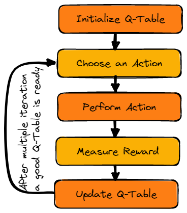
Once the Q-Table is initialized, the Q-function (seen below) is used to update it. The Q-function uses the Bellman equation and takes two inputs: state (S) and action (A). Using the equation, we can compute our Q-value for our state-action pairs. Also, note that alpha and gamma appear in this equation.

Image Source: https://www.datacamp.com/tutorial/introduction-q-learning-beginner-tutorial

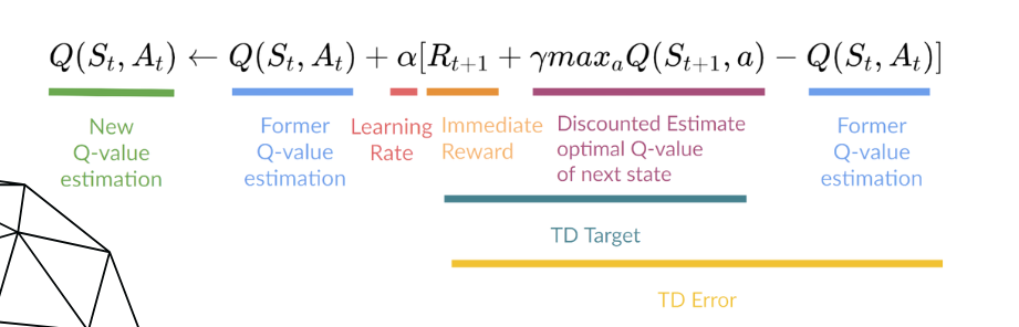
Part 3 - Alpha and Gamma

Alpha -

• The Alpha value is the learning rate for the model, and it should be somewhere in the range of 0-1. When updating the Q-Table, the higher the learning rate, the more quickly it replaces the new q value (or the more quickly it "learns"). A learning rate is a tool that can be used to find how much we keep our previous knowledge of our experience that it needs to keep for our state-action pairs. This is a hyperparameter we can tune, and we will later on in this demo.

Gamma -

• The Gamma value is the value for future reward (or the discount rate). This value should also be somewhere in the range of 0-1, and it is also a tunable hyperparameter. If the value is equal to 1, the Agent values future rewards just as much as the current reward, so very high values for gamma might not be best for learning. Conversely, a gamma of zero will cause the Agent to value only immediate rewards, which only works well in certain cases. We will explore what gamma value works best for this model later in this demo.

# This function will train our Q-Table (initialized inside the function)
# The Q-Table is initialized inside the function because we want a fresh Q-Table
# every time we run the function

# This function was created so we can tune our hyperparameters more easily

def train(ending_cell_position):
  """
  Trains the model Q-Table

  Args:
        ending_cell_position: Ending cell label (ex: 'A10')

  returns:
        mean_reward(float): the mean reward of all the episodes
        std_reward(float): the standard deviation reward of all the episodes
  """
  # This part converts the cell codename given in the argument to the row and column
  keys_end = [k for k, v in codeNames.items() if v == ending_cell_position]
  end_row_index, end_column_index = keys_end[0]

  # This will put the reward value for the goal (100) into the part of the rewards array
  # representing the cell given in the argument
  global map_rewards_new
  map_rewards_new = np.copy(map_rewards)
  map_rewards_new[end_row_index, end_column_index] = 100

  # This part initialized the Q-Table and makes sure it is accessible for other functions
  # See Part 2 above
  global table_Q
  table_Q = np.zeros((WHrows, WHcols, 4))

  # This empty list will hold the total rewards for each episode for the entire training
  episode_rewards = []

  # This is where the training begins
  for episode in range(num_episodes):

    # See Part 1 above on Epsilon Decay
    exploration_rate = min_exploration_rate + \
    (max_exploration_rate - min_exploration_rate) * np.exp(-exploration_decay_rate*episode)

    # Get an initial random start position for the robot
    row_index, column_index = start_pos()

    # This will count the total rewards in 1 episode
    total_rewards_ep = 0

    # This creates a loop that represents every step the robot takes within the episode
    # It will end if the robot reaches the goal or runs into an obstacle
    while map_rewards_new[row_index, column_index] == -1.:
        # Gets next action based on current state
        action_index = action_next(row_index, column_index, exploration_rate)

        # Gets next state based on action from above
        row_old, column_old = row_index, column_index
        row_index, column_index = location_next(row_index, column_index, action_index)

        # Calculates the reward for the new state
        reward = map_rewards_new[row_index, column_index]

        # Updating Q-Table (see Part 2 above)
        # Also see Part 3 for Alpha and Gamma Explanations
        q_old = table_Q[row_old, column_old, action_index]
        # Temporal_difference (TD) - used to estimate the expected value of Q(St+1, a)
        # by using the current state and action and previous state and action.
        TD = reward + (gamma * np.max(table_Q[row_index, column_index])) - q_old
        q_new = q_old + (alpha * TD)
        table_Q[row_old, column_old, action_index] = q_new

        # Add rewards for this step to episode total
        total_rewards_ep += reward

    # Add total rewards for this episode to list
    episode_rewards.append(total_rewards_ep)

  # Calculate the mean and std for all episodes rewards for review
  mean_reward = np.mean(episode_rewards)
  std_reward = np.std(episode_rewards)

  return mean_reward, std_reward

# This function tests our Agent with the Q-Table that was trained with the previous function

def evaluate_agent(n_eval_episodes, starting_cell_position):
  """
  Tests to see the performance of the Agent with the trained Q-Table

  Args:
        starting_cell_position: Starting cell label (ex: 'D4')
        n_eval_episodes: The number of testing episodes

  returns:
        mean_reward(float): the mean reward of all the episodes
        std_reward(float): the standard deviation reward of all the episodes
  """
  # This part converts the cell codename given in the argument to the row and column
  keys_start = [k for k, v in codeNames.items() if v == starting_cell_position]
  start_row_index, start_column_index = keys_start[0]

  # This checks if the starting cell position is valid
  if map_rewards_new[start_row_index, start_column_index] != -1.:
    print('Invalid starting position')
  else:
    # This empty list will hold the total rewards for each episode for the entire testing
    episode_rewards = []

    # This is where the testing begins
    for episode in range(n_eval_episodes):

      # Get an initial start position for the robot from start position above
      row, col = start_row_index, start_column_index

      # This will count the total rewards in 1 episode
      total_rewards_ep = 0

      # This creates a loop that represents every step the robot takes within the episode
      # It has max_steps in case you want to limit how many steps per episode
      for step in range(max_steps):

        # It will end if the robot reaches the goal or runs into an obstacle
        while map_rewards_new[row, col] == -1.:

          # Gets next action based on current state (see note below about 0 value)
          action_index = action_next(row, col, 0.)

          # Gets next state based on action from above
          row, col = location_next(row, col, action_index)

          # Calculates the reward for the new state
          reward = map_rewards_new[row, col]

          # Add rewards for this step to episode total
          total_rewards_ep += reward

      # Add total rewards for this episode to list
      episode_rewards.append(total_rewards_ep)

    # Calculate the mean and std for all episodes rewards for review
    mean_reward = np.mean(episode_rewards)
    std_reward = np.std(episode_rewards)

  return mean_reward, std_reward

Note--Epsilon's value is 0 here because when testing, we only want to exploit the best values and get the shortest path to optimize time spent getting the product

Defining Final Functions Part 2

When originally designing how I wanted these functions to work, I prioritized flexibility. I wanted to be able to have the robot start from anywhere and have the goal be anywhere (that is a legal space) in the environment. In order to achieve this, I had to be able to train a new Q-Table and run the trained Q-Table every time I ran the function with new starting and ending points.

While this is great for user ease and makes a convenient use case, there are some drawbacks. One, it is important to make sure that we try and limit the time it takes to train and how computationally intensive the training is while making it as accurate as possible. We will address this in the hyperparameter tuning section, but it is good to keep in mind for now.

Another drawback that you will see during the tuning section is consistency. Since the Q-Table has to be re-trained every time the function is run, you may get different values and, therefore, get different paths (some are shorter than others). In the tuning section, we will explore what areas we are willing to give and take on to get the desired results we want and run some tests to see how to tune our hyperparameters for consistency.

# This function converts the states from indices to the codenames

def get_codeNames_path(shortest_path):
    """
    The reverse mapping from indices of locations to the code names is done.

    Args:
          shortest_path(List): its a list of tuples containing indices

    returns:
          pathList: List of locations in final path in the form of code names
    """
    pathList = []
    for i in shortest_path:
        j=tuple(i)
        pathList.append(codeNames[j])
    return pathList

# This function brings everything together that we have learned so far
# Almost all of it we have seen in other functions, so I will not comment every line

def final_path(starting_cell_position, ending_cell_position):
    """
    Computes/prints final path of Agent/Robot

    Args:
          starting_cell_position: Starting cell label (ex: 'D4')
          ending_cell_position: Ending cell label (ex: 'A10')

    returns:
          pathList(NoneType): List of locations in final path in the form of code names
    """
    keys_start = [k for k, v in codeNames.items() if v == starting_cell_position]
    start_row_index, start_column_index = keys_start[0]

    keys_end = [k for k, v in codeNames.items() if v == ending_cell_position]
    end_row_index, end_column_index = keys_end[0]

    global map_rewards_new
    map_rewards_new = np.copy(map_rewards)
    map_rewards_new[end_row_index, end_column_index] = 100

    global table_Q

    table_Q = np.zeros((WHrows, WHcols, 4))

    for episode in range(num_episodes):

      exploration_rate = min_exploration_rate + \
      (max_exploration_rate - min_exploration_rate) * np.exp(-exploration_decay_rate*episode)

      row_index, column_index = start_pos()

      while map_rewards_new[row_index, column_index] == -1.:
        action_index = action_next(row_index, column_index, exploration_rate)

        row_old, column_old = row_index, column_index
        row_index, column_index = location_next(row_index, column_index, action_index)

        reward = map_rewards_new[row_index, column_index]

        q_old = table_Q[row_old, column_old, action_index]
        # temporal_difference
        TD = reward + (gamma * np.max(table_Q[row_index, column_index])) - q_old
        q_new = q_old + (alpha * TD)
        table_Q[row_old, column_old, action_index] = q_new

    # Creates a list object for the suggested path
    pathList=[]
    if map_rewards_new[start_row_index, start_column_index] != -1.:
        print('Invalid starting position')
    else:
        row, col = start_row_index, start_column_index
        # This holds the row/col list of the suggested path
        shortest_path = []
        shortest_path.append([row, col])
        while map_rewards_new[row, col] == -1.:
            action_index = action_next(row, col, 0.)
            row, col = location_next(row, col, action_index)
            shortest_path.append([row, col])
            # This converts the rows/cols into the codenames for user ease
            pathList=get_codeNames_path(shortest_path)
        # This creates a nice looking print statement
        for i in pathList:
          if i != pathList[-1]:
            print(i, end =" => ")
          else:
            print(i)

# This function is almost identical to the previous--it only changes the return statement to a list
# We want the return statement to be a list so we can concatenate two later

# Almost all of it we have seen in other functions, so I will not comment every line

def pre_extra_stop(starting_cell_position, ending_cell_position):
    """
    Computes/prints final path of Agent/Robot (used within extra stop function)

    Args:
          starting_cell_position: Starting cell label (ex: 'D4')
          ending_cell_position: Ending cell label (ex: 'A10')


    returns:
          pathList(List): List of locations in final path in the form of code names
    """
    keys_start = [k for k, v in codeNames.items() if v == starting_cell_position]
    start_row_index, start_column_index = keys_start[0]

    keys_end = [k for k, v in codeNames.items() if v == ending_cell_position]
    end_row_index, end_column_index = keys_end[0]

    global map_rewards_new
    map_rewards_new = np.copy(map_rewards)
    map_rewards_new[end_row_index, end_column_index] = 100

    global table_Q

    table_Q = np.zeros((WHrows, WHcols, 4))

    for episode in range(num_episodes):
      exploration_rate = min_exploration_rate + \
      (max_exploration_rate - min_exploration_rate) * np.exp(-exploration_decay_rate*episode)
      row_index, column_index = start_pos()

      while map_rewards_new[row_index, column_index] == -1.:
        action_index = action_next(row_index, column_index, exploration_rate)

        row_old, column_old = row_index, column_index
        row_index, column_index = location_next(row_index, column_index, action_index)

        reward = map_rewards_new[row_index, column_index]
        q_old = table_Q[row_old, column_old, action_index]
        # temporal_difference
        TD = reward + (gamma * np.max(table_Q[row_index, column_index])) - q_old
        q_new = q_old + (alpha * TD)
        table_Q[row_old, column_old, action_index] = q_new

    pathList=[]
    if map_rewards_new[start_row_index, start_column_index] != -1.:
        print('Invalid starting position')
    else:
        row, col = start_row_index, start_column_index
        shortest_path = []
        shortest_path.append([row, col])
        while map_rewards_new[row, col] == -1.:
            action_index = action_next(row, col, 0.)
            row, col = location_next(row, col, action_index)
            shortest_path.append([row, col])
            pathList=get_codeNames_path(shortest_path)
        # This is where we just return the list
        return pathList

# This function allows for one more argument of a middle stop in the path

# We use the previous function so we can concatenate the two lists together to make
# a final path

def extra_stop(starting_location, intermediary_location, ending_location):
    """
    Computes/prints final path of Agent/Robot with extra stop

    Args:
          starting_cell_position: Starting cell label (ex: 'D4')
          intermediary_location: intermediary cell label (ex: 'D6')
          ending_cell_position: Ending cell label (ex: 'A10')

    returns:
          pathList(NoneType): List of locations in final path in the form of code names
    """
    # Here we run the pre_extra_stop() function twice with the intermediary_location
    # in the middle. We also use [1:] so the intermediary_location is not listed twice
    final = pre_extra_stop(starting_location, intermediary_location) + pre_extra_stop(intermediary_location, ending_location)[1:]
    for i in final:
      if i != final[-1]:
        print(i, end =" => ")
      else:
        print(i)

Training the model and Hyperparameter Tuning

In this section, we will tune our hyperparameters to see what values work best for this model in training and testing. This is especially important because (as I mentioned earlier) when we run the final function, we will train a new Q-Table and run the newly trained Q-Table every time.

In order to try and fully discover how this affects our model, we will be exploring the hyperparameter tuning in two sections—one that will focus on how each parameter affects the training numbers of the model. The other section will focus on consistency when running the testing functions with the same inputs many times with slightly different Q-Tables each time.

We will pay special attention to the hyperparameters num_episodes, alpha, exploration_decay_rate, and gamma. Please reference the explanations above to understand why we would want to tune alpha, exploration_decay_rate, and gamma. We want to tune num_episodes because that is one of the main metrics we can control that affects how long it takes to train our model and, therefore, how long it will take to run our final function. When we get to the consistency section, we have to weigh the pros and cons of the value of a quick vs. accurate function.

Seeing how Hyperparameters affect model

# These are two parameters that could be tuned for the testing

# This represents the number of episodes it will train
n_eval_episodes = 100

# This represents the max steps the robot can take in 1 episode
# This is not needed as much for this demo, but it could be useful if it was larger
max_steps = 100

Note--even though we are mostly paying attention to the training values at this point, it is still helpful to see how it performs in testing.

Test 1 (a)

• Initial test (nothing to change)

# These are the main hyperparameters we will be tuning
# In particular, num_episodes, alpha, exploration_decay_rate, and gamma

num_episodes = 5000

alpha = 0.1 # learning_rate
gamma = 0.99 # discount_rate

exploration_rate = 1 # epsilon
max_exploration_rate = 1
min_exploration_rate = 0.01
exploration_decay_rate = 0.001 # decay rate

train('E10')

(48.941000000000003, 56.095517815597354)

evaluate_agent(n_eval_episodes, 'H1')

(83.0, 0.0)

What did we learn?

This is a good baseline to see how the parameters affect the model when changed.

Test 2 (a)

• What did we change?
  • num_episodes from 5000 to 10000

num_episodes = 10000

alpha = 0.1 # learning_rate
gamma = 0.99 # discount_rate

exploration_rate = 1 # epsilon
max_exploration_rate = 1
min_exploration_rate = 0.01
exploration_decay_rate = 0.001 # decay rate

train('E10')

(67.131600000000006, 46.710117548985039)

evaluate_agent(n_eval_episodes, 'H1')

(85.0, 0.0)

Note--The 85 we see above is 100-15, which represents the reward of 100 subtracted by the -1 * 15 squares it took to get there (it does not count the first square). As a spot check, this makes sense. Given that this is the most efficient number (so far), we want to get as close as possible to this when tuning in training--without getting too close because we want the model to explore enough in the beginning.

What did we learn?

Increasing the num_episodes definitely increases the overall accuracy of the training (and testing--85 is better than 83). However, this takes more time than a lower number, and it is possible that we do not need all that training for the testing to be accurate. We can also potentially get accurate training numbers by tuning the other hyperparameters. One potential reason the accuracy likely increases so much is that, towards a larger portion of the end, the epsilon rate is exploiting more. We will continue to explore and see what we find.

Test 3 (a)

• What did we change?
  • num_episodes from 10000 to 1000
  • exploration_decay_rate from 0.001 to 0.01 (the reason is that the function gets hung up with such a "small" number of episodes at the smaller decay rate)
  • from here on, we will keep the decay rate at 0.01 until the next section

num_episodes = 1000

alpha = 0.1 # learning_rate
gamma = 0.99 # discount_rate

exploration_rate = 1 # epsilon
max_exploration_rate = 1
min_exploration_rate = 0.01
exploration_decay_rate = 0.01 # decay rate

train('E10')

(54.226999999999997, 57.524077315503291)

evaluate_agent(n_eval_episodes, 'H1')

(85.0, 0.0)

What did we learn?

Decreasing the num_episodes to 1000 decreases the accuracy of the training, but it also decreases the time the function takes to run. Also, the testing was still the best version so far at this number, so it may end up being worth it to keep the training episodes lower, especially after we tune the other hyperparameters.

It is also worth noting that we had to make the epsilon decay rate larger when the num_episodes is smaller because otherwise, the functions get stuck. This makes sense because there are fewer episodes for epsilon to decay. The same is true that the larger decay rate does not work as well in this case with the larger number of episodes.

Test 4 (a)

• What did we change?
  • gamma from 0.99 to 0.7

num_episodes = 1000

alpha = 0.1 # learning_rate
gamma = 0.7 # discount_rate

exploration_rate = 1 # epsilon
max_exploration_rate = 1
min_exploration_rate = 0.01
exploration_decay_rate = 0.01 # decay rate

train('E10')

(50.228000000000002, 60.133651277799522)

evaluate_agent(n_eval_episodes, 'H1')

(85.0, 0.0)

What did we learn?

Based on this test, we should try and keep gamma as high as possible.

Test 5 (a)

• What did we change?
  • alpha from 0.1 to 0.5

num_episodes = 1000

alpha = 0.5 # learning_rate
gamma = 0.99 # discount_rate

exploration_rate = 1 # epsilon
max_exploration_rate = 1
min_exploration_rate = 0.01
exploration_decay_rate = 0.01 # decay rate

train('E10')

(59.908999999999999, 52.762796732167253)

evaluate_agent(n_eval_episodes, 'H1')

(85.0, 0.0)

What did we learn?

In this test, we learned that compared to Test 3, it is better if the alpha is higher.

Test 6 (a)

• What did we change?
  • gamma from 0.5 to 0.99

num_episodes = 1000

alpha = 0.99 # learning_rate
gamma = 0.99 # discount_rate

exploration_rate = 1 # epsilon
max_exploration_rate = 1
min_exploration_rate = 0.01
exploration_decay_rate = 0.01 # decay rate

train('E10')

(61.021999999999998, 51.91371221556016)

evaluate_agent(n_eval_episodes, 'H1')

(85.0, 0.0)

What did we learn?

In this final test in this section, we confirm that the model performs fairly well when alpha is high. We will explore more in the next section.

Exploring Consistency

In this section, we will be exploring the distribution of path lengths given by running the function pre_extra_stop() 100 times. Our goal is to have the majority of responses be the shortest path and have the fewest number of different paths suggested.

Defining Function and setting up for tests

# Number of times we want to run our final function

num_tests = 100

# This function takes the input of num_tests to check the path length each time
# the final function pre_extra_stop is run (I chose that function since you can count in lists)

# The dictionary then sorts and counts each type of length that comes from function
# pre_extra_stop during the tests

def my_test_function(num_tests, starting_cell_position, ending_cell_position):
  """
    Checks the distribution of suggested path lengths by running pre_extra_stop()
    num_tests amount of times

    Args:
          num_tests: Number of times to run pre_extra_stop() function
          starting_cell_position: Starting cell label (ex: 'D4')
          ending_cell_position: Ending cell label (ex: 'A10')

    returns:
          dict(dictionary): Dictionary of path lengths with lengths as key and
                            frequency as value
  """
  list = []

  for i in range(num_tests+1):
    list.append(len(pre_extra_stop(starting_cell_position, ending_cell_position)))

  dict = {i:list.count(i) for i in list}

  return dict

Note--The function my_test_function() can take a while to run depending on num_episodes

Note--The numbers I mention in the subsequent sections may be slightly off due to the nature of testing. However, the overall ideas should still be accurate regardless.

Running Tests on Consistency

Test 1 (b)

• We are going to start with where we left off in the previous section

num_episodes = 1000

alpha = 0.99 # learning_rate
gamma = 0.99 # discount_rate

exploration_rate = 1 # epsilon
max_exploration_rate = 1
min_exploration_rate = 0.01
exploration_decay_rate = 0.01 # decay rate

my_test_function(num_tests, 'H1', 'E10')

{19: 38, 17: 60, 21: 3}

What did we learn?

Here, we start to see the problem. In the 100 times the pre_extra_stop() function was run, it only got the actual shortest path 56 of those times. The other path lengths are close, but ideally, we would want a more likely chance of getting the shortest path every time we run the function.

Test 2 (b)

• What did we change?
  • We increased the num_episodes back to 10000
  • We changed the decay rate back to 0.001

num_episodes = 10000

alpha = 0.99 # learning_rate
gamma = 0.99 # discount_rate

exploration_rate = 1 # epsilon
max_exploration_rate = 1
min_exploration_rate = 0.01
exploration_decay_rate = 0.001 # decay rate

my_test_function(num_tests, 'H1', 'E10')

{17: 93, 19: 8}

What did we learn?

In this test, we learned that it performed much better when there were more episodes in testing. There were fewer path options, and it got the shortest path 91 out of 100 times. However, this comes at the expense of a speedy function later on. Let’s see if we can get an almost as good version that would be faster.

Test 3 (b)

• What did we change?
  • We dropped the num_episodes down to 2500 to try and speed up the function
  • We changed the decay rate to 0.01

num_episodes = 2500

alpha = 0.99 # learning_rate
gamma = 0.99 # discount_rate

exploration_rate = 1 # epsilon
max_exploration_rate = 1
min_exploration_rate = 0.01
exploration_decay_rate = 0.01 # decay rate

my_test_function(num_tests, 'H1', 'E10')

{17: 72, 19: 26, 21: 3}

What did we learn?

This test performed slightly better than Test 1 (b), but not by a large margin. Plus, it performed much worse than the 10,000 episodes test. However, it would run faster, so let’s run another test to see if we can get 2500 to improve.

Test 4 (b)

• What did we change?
  • We changed the decay rate back to 0.001

num_episodes = 2500

alpha = 0.99 # learning_rate
gamma = 0.99 # discount_rate

exploration_rate = 1 # epsilon
max_exploration_rate = 1
min_exploration_rate = 0.01
exploration_decay_rate = 0.001 # decay rate

my_test_function(num_tests, 'H1', 'E10')

{17: 82, 19: 19}

What did we learn?

Decreasing the decay rate really helped in this case. The final breakdown was that it got the shortest path 84 out of the 100 times. While this is not quite as good as the 10,000 episodes, this will take a lot shorter to run when used in the end.

Running the Functions and Visuals

Below are the best versions of the hyperparameters, given the tradeoffs.

# These are the tuned hyperparameters that were decided earlier

num_episodes = 2500

alpha = 0.99 # learning_rate
gamma = 0.99 # discount_rate

exploration_rate = 1 # epsilon
max_exploration_rate = 1
min_exploration_rate = 0.01
exploration_decay_rate = 0.001 # decay rate

How does this tie back into our problem?

If we remember our Case Study from the Presentation, making a system similar to this one could help companies like Stitch Fix (or Amazon) find the optimal pathways for their robots to collect items for packing. The goal of finding the shortest path is to reduce time and increase efficiency so they can do more business. Also, having autonomous robots able to find pathways through a warehouse (despite obstacles) can free up people to do other tasks or their tasks more efficiently.

Note--Since there are multiple valid solutions sometimes the solution the code runs and the picture may not be the same. However, the pictures show a path that the code has come up with before.

Here is what it looks like when running the function!

final_path('D4', 'A10')

D4 => C4 => B4 => A4 => A5 => A6 => A7 => A8 => A9 => A10

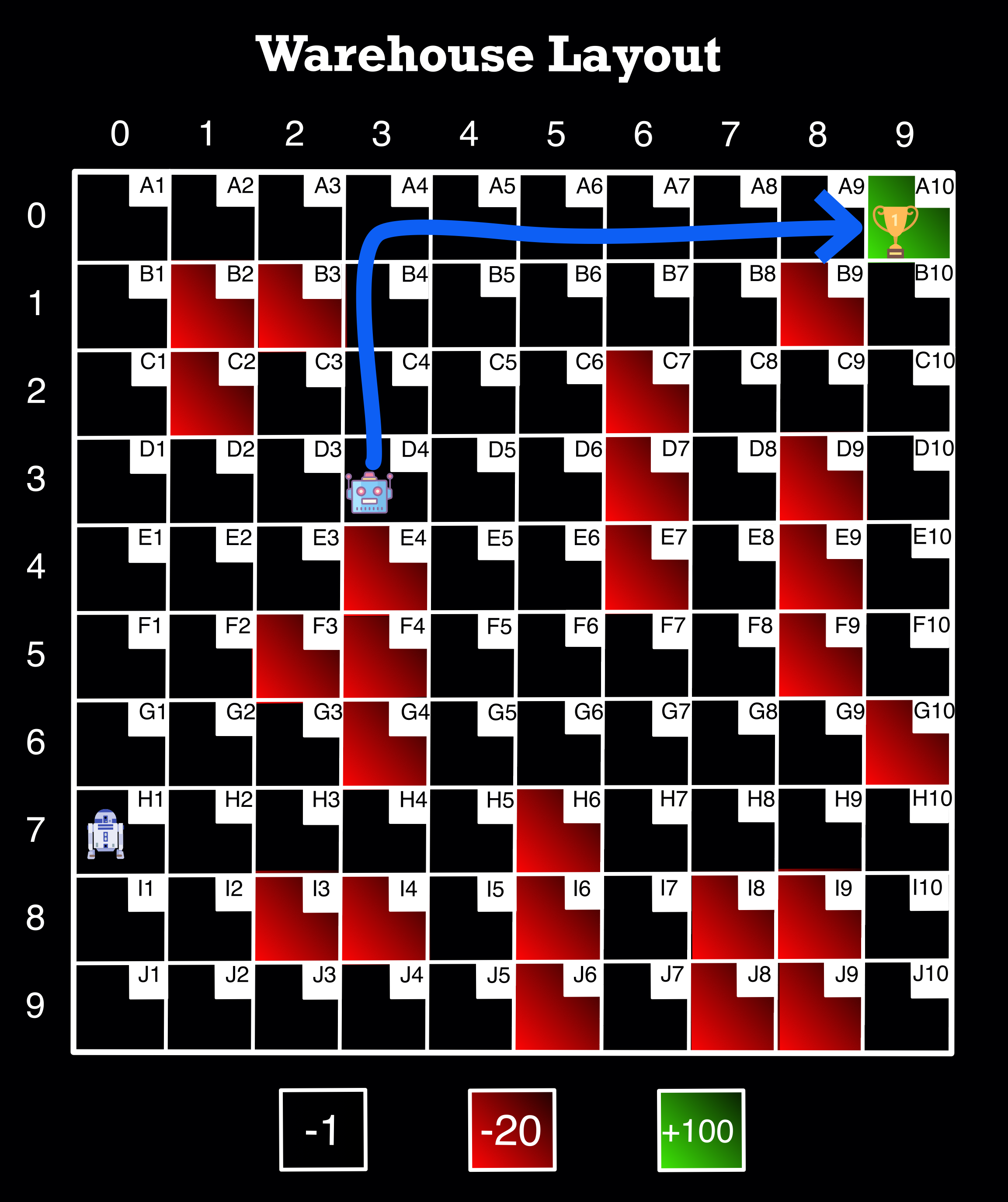
Image Source: Author

final_path('D1', 'E10')

D1 => D2 => D3 => C3 => C4 => B4 => B5 => B6 => B7 => B8 => C8 => C9 => C10 => D10 => E10

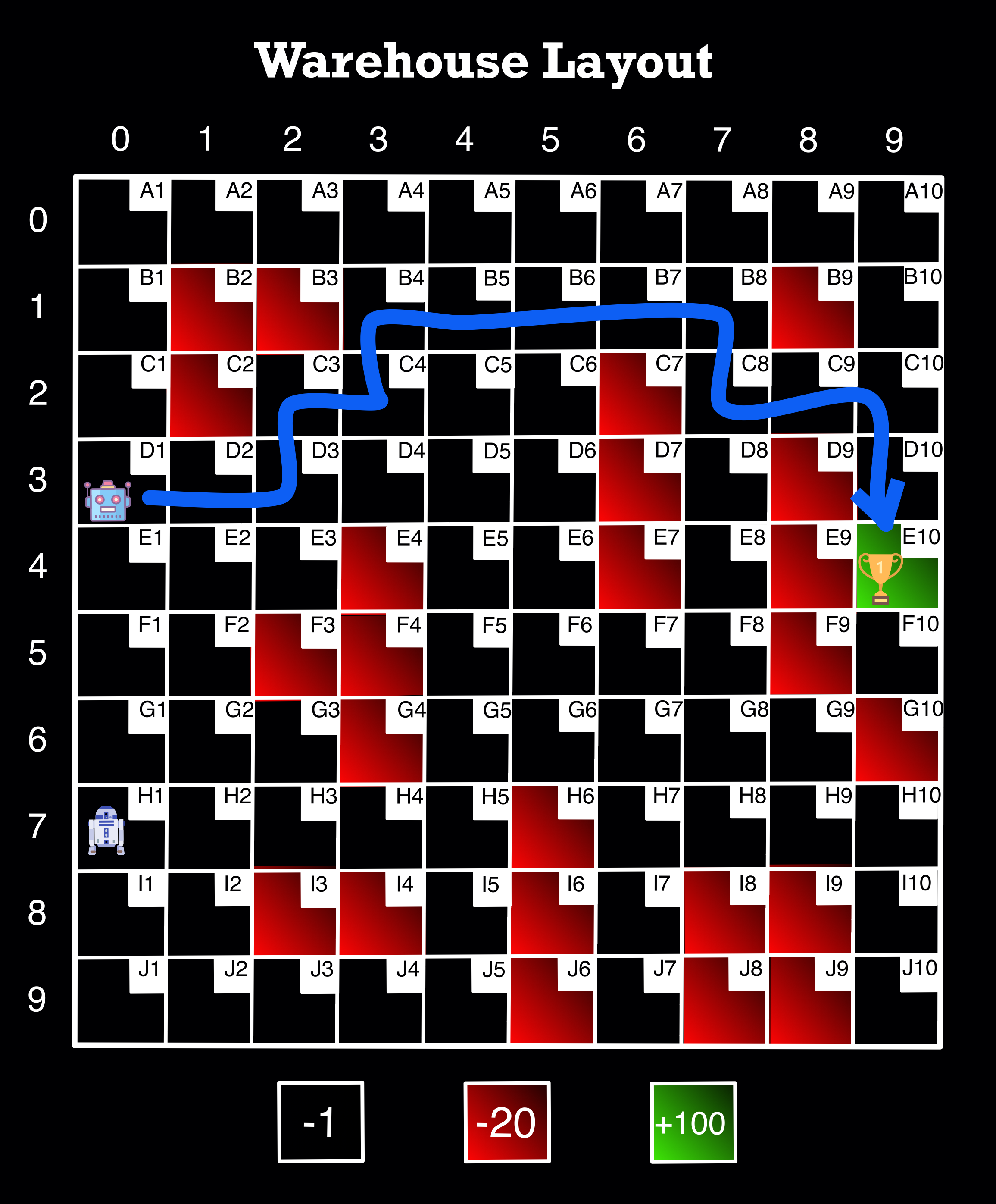
Image Source: Author

extra_stop('D4', 'D6', 'A10')

D4 => D5 => D6 => C6 => B6 => A6 => A7 => A8 => A9 => A10

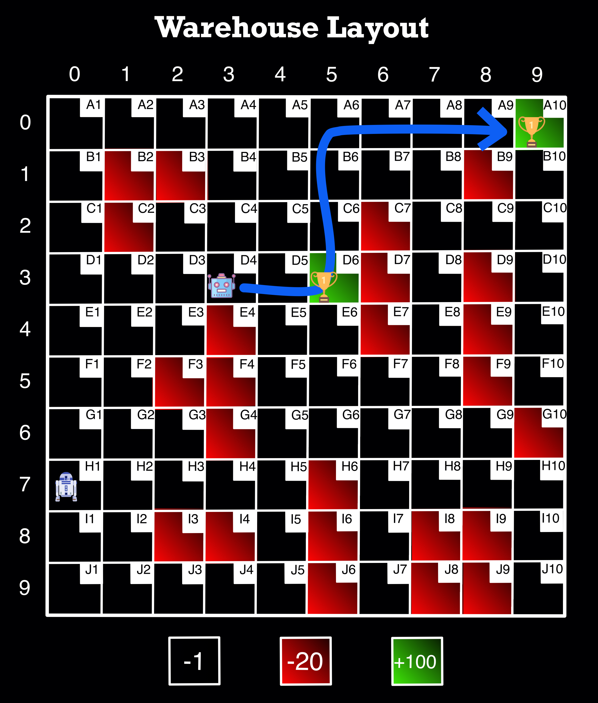
Image Source: Author

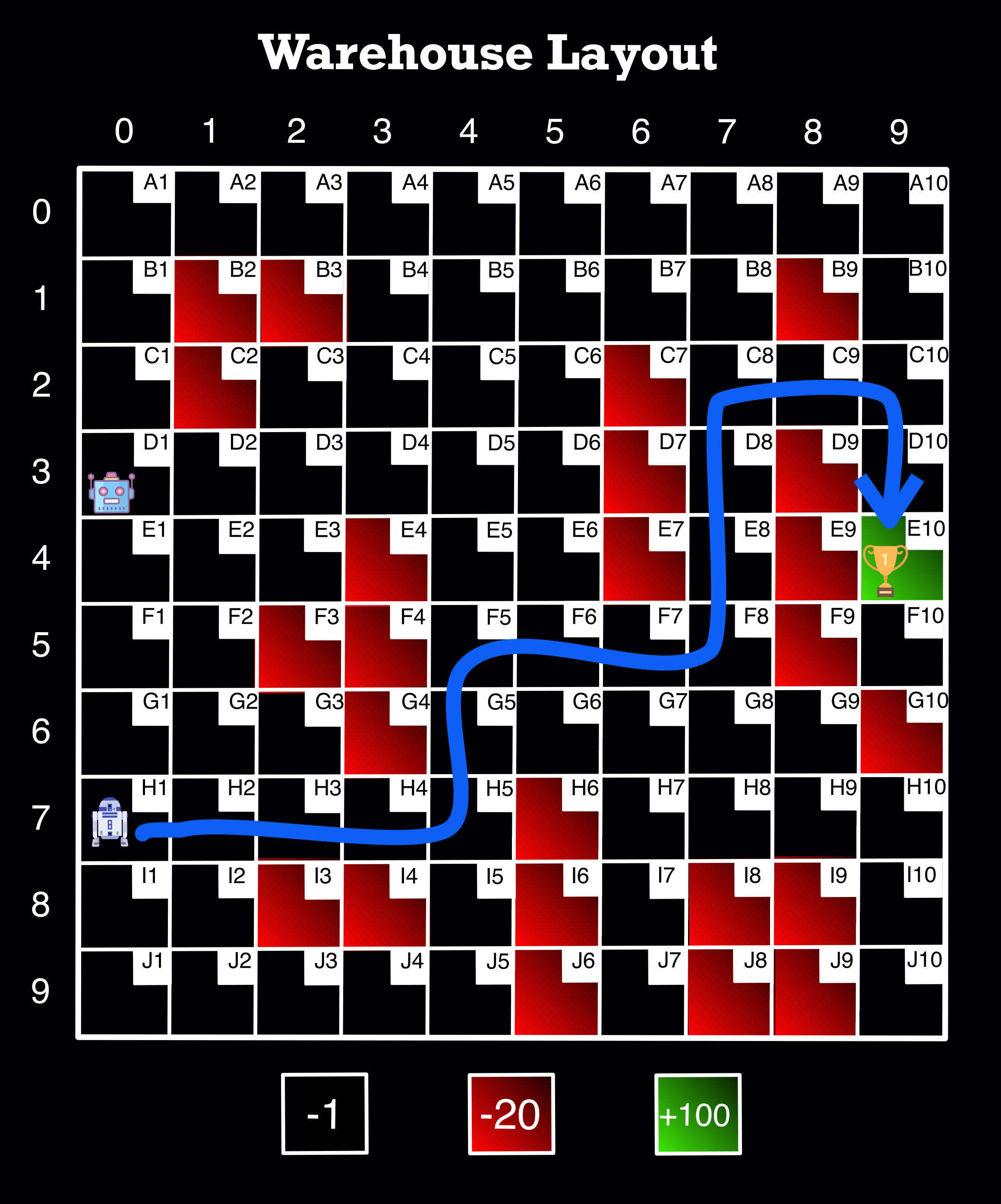
final_path('H1', 'E10')

H1 => H2 => H3 => H4 => H5 => G5 => F5 => F6 => F7 => F8 => E8 => D8 => C8 => C9 => C10 => D10 => E10

Image Source: Author

extra_stop('H1', 'H7', 'E10')

H1 => H2 => H3 => H4 => H5 => G5 => G6 => G7 => H7 => G7 => F7 => F8 => E8 => D8 => C8 => C9 => C10 => D10 => E10

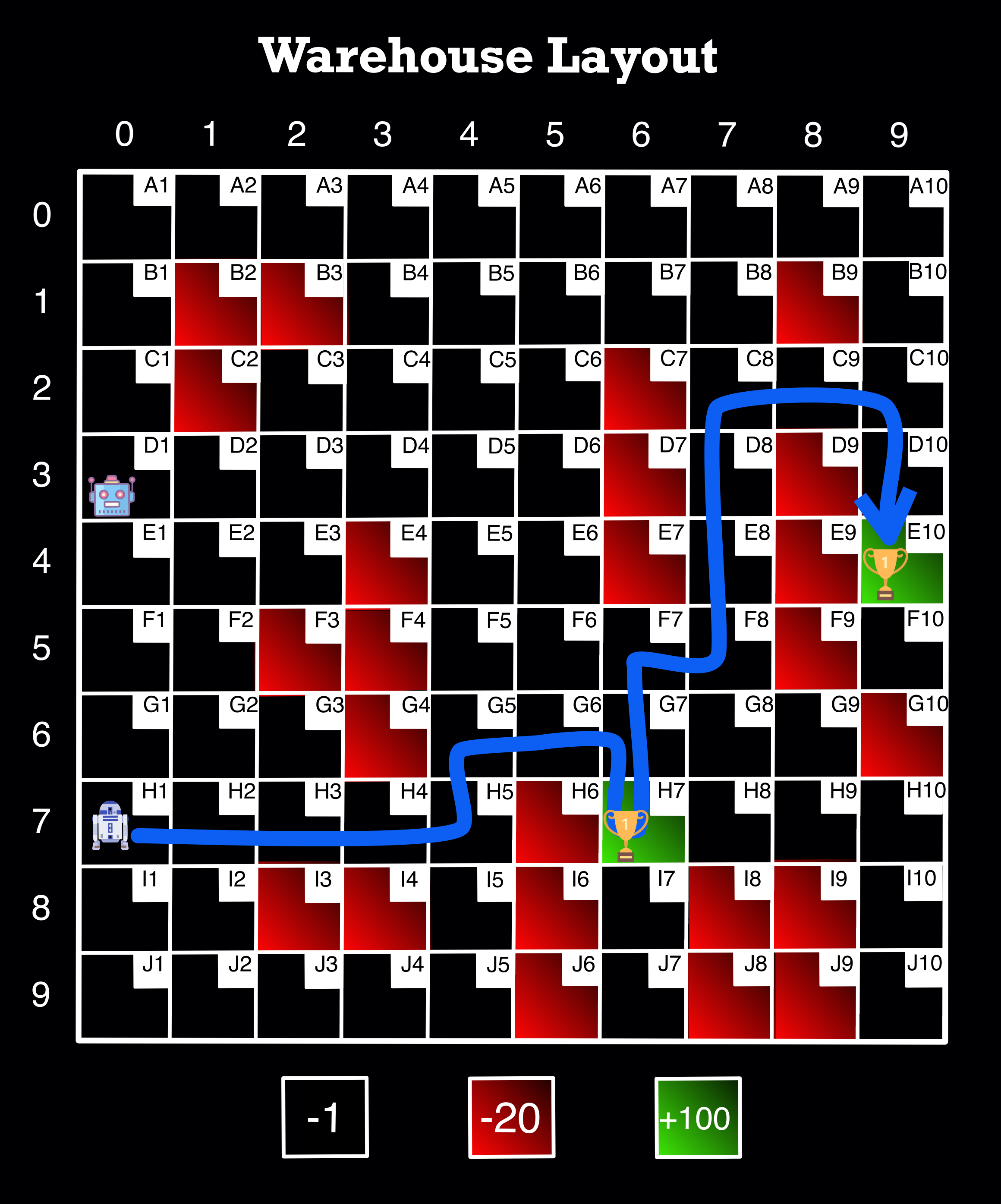
Image Source: Author

Main Sources for this Demo (see presentation for full citation list):

Reinforcement Learning 8: Pick and Place Robot in an E-Commerce Store Warehouse i.e. Q-Learning in Action

Get Started With Q-Learning With Python: How To Automatize A Warehouse Robot

An Introduction to Q-Learning: A Tutorial For Beginners